Unsteady free convection flow of Casson fluid over an unbounded upright plate subject to time dependent velocity \(U_{o}f(t)\) with constant wall temperature has been carried out. By introducing dimensionless variables, the general solutions are obtained by Laplace transform method. The solution corresponding to Newtonian fluid for \(\gamma \rightarrow \infty\) is obtained as a limiting case. Exact solutions corresponding to (i) \(f(t)=f H(t)\), (ii) \(f(t)=f t^{a}\), \(a > 0 \) (iii) \( f(t)=f H(t)cos(\omega t)\) are also discussed as special cases of our general solutions. Expressions for shear stress in terms of skin friction and the rate of heat transfer in the form of Nusselt number are also presented. Velocity and temperature profiles for different parameters are discussed graphically.Free convection; Time depending velocity; Exact solutions; Casson fluid; Vertical plate.
For the last few decades Casson fluid become popular among researchers due to its importance in the field of food processing, drilling muds, metallurgy, different oils and suspensions and in bioengineering. Casson fluid is assessed as a non-Newtonian fluid because of its rheological traits. These characteristics display shear stress-strain relationships which might be extensively one of a kind from Newtonian fluids. Unlike Newtonian fluids, these fluids are described by a nonlinear relationship between the stress and the rate of strain. These fluids can be complicated when compare to Newtonian fluids and can not be described by Navier-Stokes equations. The properties of non-Newtonian fluids’s flow can be very critical due to the fact they play an extensive part in engineering and industry. In numerous regions of biorheology, geophysics, and chemical and petroleum industries such interest is encouraged because of their considerable application. As a result the research on non-Newtonian fluids have now increasingly grown and becomes a more attractive subject matter of modern studies in this discipline. It is therefore important to focus the study of Casson fluid.
As non-Newtonian fluids are complicated in nature, they are very hard to explain by a single constitutive relation. So different constitutive equations and expressions are established to discuss their behavior. Second grade, Maxwell, Power law, viscoplastic, Jeffrey, Bingham plastic, Brinkman, Oldroyd-B and Walters-B are some examples of these models [1, 2, 3, 4, 5, 6, 7, 8, 9]. Recently, Casson model has attracted the attention of the researchers.
Casson properties were firstly described by Casson [10] for the flow charecteristics of pigment oil solutions of the printing ink. So, to produce the motion, the shear stress of Casson fluid must be greater than the yield shear stress, and if not then fluid acts like a solid. Such kind of fluids are considered as a viscous fluid with high viscosity [11]. At zero rates of shear, Casson fluid has a boundless viscosity and a yield stress below which flow cannot be occurred. Casson model exhibits the solid and liquid phases [12]. In fluid dynamics, the study of Casson fluids become very important due to its various applications in pharmaceutical products, paints, lubricants sewage sludge, jelly, tomato sauce, honey, soup, and blood.
Blood can also be handled as Casson fluid because of the presence of numerous materials inclusive of protein, fibrinogen, globulin in aqueous
base plasma and human red blood cells [1, 14]. Afterwards, a lot of work is done on Casson fluid for different flow conditions and combinations by researchers [15, 16, 17, 18, 19, 20, 21, 22, 23, 24]
Free convection takes place when the medium transferring the heat is being inspired to move by the heat itself. This happens both, in the case of gases because the medium expands as it heats up and also because buoyancy causes the warmer fluid to rise. Convection is of three types namely free, mixed and force. Amongst them free convection is important in many engineering applications including an example of automatic control systems consist of electrical and electronic components, regularly subjected to periodic heating and cooled by free convection process.
Many scientists studied the free convection phenomena for different situations [25, 26, 27, 28, 29, 30, 31].
Free convection phenomena has wide applications in engineering, industrial, nuclear reactors technology, geophysics, geothermal energy, construction insulation, food processing and aeronautics.
Mixed convection stagnation-point flow of Casson fluid with convective boundary conditions is examined by Hayat et al. [32]. Mustafa et al. [33] investigated the unsteady flow and heat transfer of a Casson fluid over a moving flat plate. Rao et al. [34] considered the thermal and hydrodynamic slip conditions on heat transfer flow of a Casson fluid over a semi-infinite upright plate.
Heat transfer flow of a Casson fluid over a permeable shrinking sheet with viscous dissipation was considered by Qasim and Noreen [35]. Exact solutions for unsteady free convection flow of
Casson fluid over an oscillating vertical plate with constant wall temperature and unsteady MHD free convection flow of Casson fluid past over an oscillating vertical plate embedded in a porous medium are studied by Sharidan Shafie et al. [36, 37]. Unsteady boundary layer flow and heat transfer of a Casson fluid over an oscillating upright plate with Newtonian heating was investigated by
Abid Hussanan et.al. [38]. Natural convection flow of a non-Newtonian Casson
fluid over an upright stretching plane with mass diffussion is examined by A. Mahdy [39].
In all of the above studies the solutions of Casson fluid are obtained by using either approximate method or any numerical scheme. There are very few cases in
which the exact analytical solutions of Casson fluid are obtained. These solutions are very few when Casson fluid in free convection flow with constant wall temperature is considered. However, the Casson fluids model in the presence of heat transfer, is an vital research area as it is frequently used to process molten chocolate, toffee and blood situations.
Motivated by the above investigations, the present analysis is focused on the study of jerky and unformed free convection flow of Casson fluid past an upright
plate subject to the time dependent velocity with constant wall temperature. Analytical as well as numerical results for skin friction and Nusselt number are obtained. Also we will discuss the effects of different parameters on the velocity and temperature profiles graphically.
2. Statement of the problem
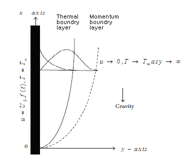
Consider the impact of heat diffusion on jerky and unformed boundary layer flow of an incompressible Casson fluid over an unbounded flat plate located at \(y=0\). The flow is restricted to \(y>0\), where the \(x\) coordinate is taken along the plate in the upright direction and \(y\) is normal direction to the surface. Let us suppose that, initially at \(t=0\), the fluid and plate are stationary with invariant temperature \(T_\infty\). When time is \(t=0^+\), the plate starts moving with time dependent velocity \(U_{o}f(t)\) in its plane where \(U_o\) is the characteristics velocity. At the same time, the plate temperature raised to constant temperature \(T_w\).
Figure 1. Coordinate system and Physical model
The rheological equation of the state for an isotropous and incompressible flow of a Casson fluid can be written as, [19,31]
$$\tau=\tau_0+\mu\gamma^\star$$,
where \(\tau\) is the shear stress, \(\tau_{0}\) is the Casson yield stress, \(\mu\) is the
dynamic viscosity, \(\gamma^{*}\) is the shear rate, \(\pi=e_{ij} \ e_{ij}\) and \(e_{ij}\) is the \((i,j)^{th}\) component of the deformation rate, \(\pi\) is the product of the component of deformation rate with itself, \(\pi_{c}\) is a critical value of this product based on model, \(\mu_{\beta}\) is plastic dynamic viscosity of non -Newtonian fluid and \(p_{y}\) is the yield stress of fluid. Under the conditions along with the assumption that the viscous dissipation term in the energy equation is neglected, we get the following set of partial differential equations [36],
In the next, the
solution of coupled partial differential equations (2) and (3) with the initial
and boundary conditions will be determined by means of Laplace transforms.
3. Solution of the problem
In order to solve the above problem, we firstly introduce the following dimensionless
quantities.
where \(\textrm{Pr}=\frac{\mu c_{p}}{R}, \textrm{Gr}=\frac{\nu\beta(T_{w}-T_{\infty})}{U_{o}^{3}},\)
and \(\gamma=\frac{\mu_{\beta}\sqrt{2\pi c}}{p_{y}},\) are Prandtl number, Grashof number and Casson Parameter respectively. In order to solve the initial-boundary value problem (7 – 11), we use the Laplace transform technique.
The Laplace transform of eq. (7) and (8) is given as
where \( \bar{u}(y,q),\ \bar{\theta}(y,q)\) and \(\bar{F}(q)\) are Laplace transform of the functions \( u(y,t), \theta(y,t)\) and \(f(t)\) respectively.
The solution of eq. (13) subject to \( (14)_{2}\) , \((15)_{2}\) is given by
where \( b= \frac{a \textrm{G}_{r}}{Pr-a}, \) \(\textrm{Pr}\neq a \) and \( a= \frac{\gamma}{1+\gamma}\).
By inverting eq.(16) , we have the expression for the non dimensional temperature
corresponds to mechanical part. The non-dimensional skin friction is calculated from the
velocity field (21), using the relation
\(\tau= -\mu\left(1+\frac{1}{\gamma}\right)\frac{\partial u}{\partial y}|_{y=0}\)
Case 2: In the absence of free convection the corresponding buoyancy forces are zero i.e \((Gr=0)\) due to the differences in temperature gradient. This shows that the thermal part of the velocity is zero and flow is governed only by mechanical part of the velocity.
Let us firstly consider \(f (t) = f H(t)\) where \(f\) is a dimensionless constant and \(H(.)\) is the unit Heaviside
step function. In this case, after time \(t = 0^{+}\), the infinite plate starts to move with constant velocity. The thermal
component of velocity \(u_{t}(y, t)\) remain unchanged, while \(u_{m}(y, t)\) takes the simplified form
when \(a=1\) the plate starts to move with constant acceleration. The corresponding expression of the mechanical component \(u_{m 1}(y, t)\), resulting from (31), is
This is the mechanical component of the fluid velocity
in the motion induced by an infinite oscillating plate. It can be written
as a sum between steady-state and transient solutions:
When the direction and magnitude of flow is constant with time throughout the entire domain steady state flow occurs. Whereas, transient flow occurs if the magnitude and direction of the flow varies with time.
When \(\gamma\rightarrow\infty\), we obtained well known results in the absence of free convection identical to Fetecau ([40], see (10)) when \(U=1\), \(\nu=1\) and \(f=1\).
On evaluating eq. (34),
For the sake of conclusion of the behaviour of dimensionless temperature and velocity fields and to get some tangible
perception of the obtained solutions, successive numerical calculations were accomplished for different values of
pertinent constraints like Prandtl number Pr, Grashof number Gr, time \(t\) and Casson parameter \(\gamma\). Numerical calculations of Nusselt number and skin friction are presented in tables 1 and 2 for different constraints. Figure 2-8 correspond to the case when the plate
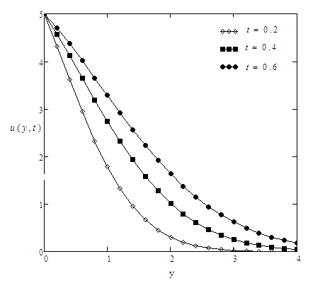
applies a constant velocity to the fluid. Figure 2 illustrates the consequence of time \(t\)
on the velocity. It is depicted that the velocity is an increasing function of time \(t\). Figure 3 shows
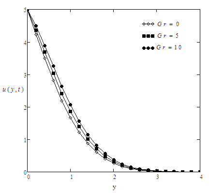
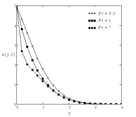
the profiles of velocity for different values of Gr which states that velocity is decreasing with decreasing values of \(Gr\). In Figure 4, consequences of Prandtl number upon velocity profiles are shown. This indicates that velocity of the fluid is
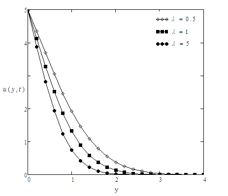
decreasing with increasing Prandtl number. In Figure 5, effect of Casson parameter upon velocity profiles are discussed.
It is noted that
for increasing values of \(\gamma\), velocity decreases. It is also seen that with
increasing Casson parameter velocity boundary
layer thickness shorter. It is further noticed from this graph
that when the Casson parameter $\gamma$ is large enough, that is,
\(\gamma \rightarrow \infty\), the non-Newtonian behavior vanishes and the
fluid acts just like a Newtonian fluid. Therefore, for Casson fluid, the velocity
boundary layer thickness is greater as compare to the
Newtonian fluid.
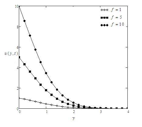
Figure 6 interprets
the profiles of velocity for different values of \(f\). It is
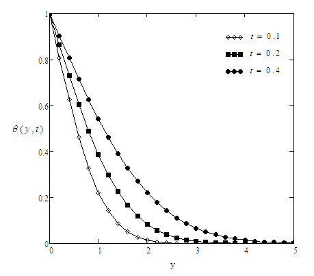
noticed that velocity increases when \(f\) is increased. The consequence of time t on temperature profiles
can be seen in Figure 7. As expected, when the time is increased, the temperature is also increased. This graphical behavior of temperature is in good
accordance with the corresponding boundary conditions of
temperature profiles as shown in (8-9).
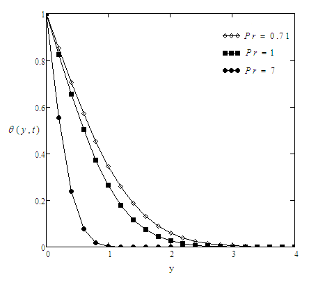
Figure 8 illustrates the effect of specific values of Prandtl number such as \(Pr = 0.71\) (air), \(Pr = 7.0\) (water),
and \(\textrm{Pr} = 25\) (honey) on the temperature profile. It can be seen that temperature falls as the values of Prandtl number Pr are increased.
It is depicted from the diagram that near the plate, thickness of thermal boundary layer
is largest. It is decreased when distance from the leading edge is increased and ultimately it is approached to zero.
It can be seen that the value of temperature is smaller for honey as compared to water and air. The reason behind this is as Prandtl
number increases thermal conductivity of the fluid decreases which reduces the thickness of thermal boundary layer.
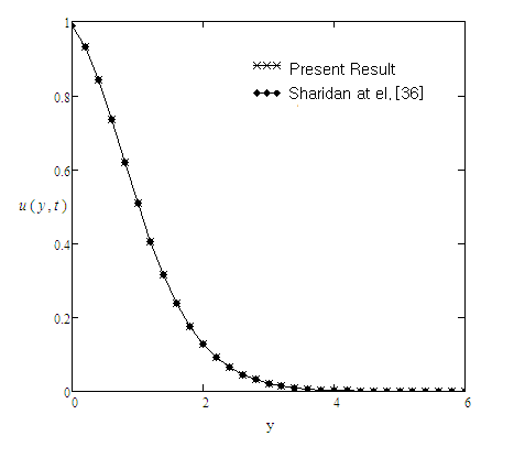
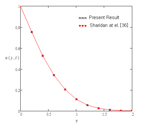
For the sake of correctness and verification, obtained results are tallied with those of Fetecau et al. [40] and Sharidan et al. [36]. Figure 9 shows that our results (37) are in good accordance with those obtained by Sharidan et al. ([36], see (14)). This confirms the accuracy of our obtained results. It is also found from Figure 10, that our limiting
solutions (35) are identical the results obtained by Fetecau
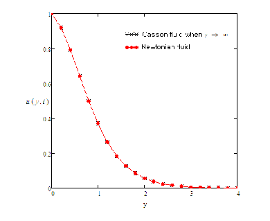
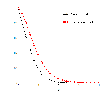
et al. ([40], see (9) and (11)) and by Sharidan et al.([36], see (24)). Figure 11 illustrates the fact that our results (25) for Newtonian fluid when fluid is moving with constant velocity are identical to (30) when \(\gamma \rightarrow \infty\). We have also compared the velocity profiles for Newtonian and Casson fluids in Fig. 12. It is observed that Casson fluids are slower than Newtonian fluids. It is cleared from the figure that Newtonian fluids have greater velocity as compare to the Casson fluids. Table 1 indicates that with increasing Pr, Nusselt number is increasing whereas it decreases with increasing t. From Table 2, it is found that skin friction increases with increasing \(Pr\) and \(f\) whereas it increases with decreasing \(Gr\), \(\gamma\) and \(t\).
Figure 2. Profiles of the velocity for different values of \(t\), when \(Pr=0.3\), \(f=5\), \(Gr=3\), and \(\gamma=0.6\).Figure 3. Profiles of the velocity for different values of \(Gr\), when \(\textrm{Pr}=0.3\), \(f=5\), \(\gamma=0.6\), and \(t=0.2\).Figure 4. Profiles of the velocity for different values of \(\textrm{Pr}\), when \(\textrm{Gr}=3\), \(f=5\), \(\gamma=0.6\), and \(t=0.2\).Figure 5. Profiles of the velocity for different values of \(\gamma\), when \(\textrm{Pr}=0.3\), \(f=5\), \(\textrm{Gr}=3\), and \(t=0.2\).Figure 6. Profiles of the velocity for different values of \(f\), when \(\textrm{Pr}=0.3\), \(\gamma=0.6\), \(\textrm{Gr}=3\), and \(t=0.2\).Figure 7. Profiles of the temperature for different values of \(t\), when \(\textrm{Pr}=0.3\).Figure 8. Profiles of the temperature for different values of \(\textrm{Pr}\), when \(t=0.4\).Figure 9. Comparison of the present results (see (37)) with those obtained by Sharidan et al. [36] (see (14)) and, when \(t = 0.2\), \(\textrm{Gr} = 3\), \(a = 0.375\), \(f=1\) and \(\textrm{Pr}=0.15\).Figure 10. Comparison of the present results (see (35)) with those obtained by Fetecau et al. [40] (see (8) and (10)) Sharidan et al. [36] (see (24)) and, when \(t = 0.2\), \(\textrm{Gr} = 0\), \(a = 1\), \(U = 1\), \(f=1\) and \(\nu = 1\).Figure 11. Comparison of the velocity profiles for Casson fluid when \(\gamma\rightarrow\infty\) (25) and Newtonian fluid (30), when plate moves with constant velocity and \(a=1\), \(f=1\), \(\textrm{Pr}=0.3\), \(\textrm{Gr}=2\) and \(t=0.3\).Figure 12. Comparison of the velocity profiles for Casson fluid (30) and Newtonian fluid (25) when plate starts to move with constant velocity and \(\textrm{Gr}=2\), \(f=1\), \(\textrm{Pr}=0.3\) and \(t=0.3\).
Table 1. Nusselt number Variations
\(Pr\)
\(t\)
\(Nu\)
\(0.3\)
\(0.3\)
\(0.564\)
\(0.3\)
\(0.5\)
\(0.437\)
\(0.71\)
\(0.3\)
\(0.868\)
\(0.71\)
\(0.5\)
\(0.672\)
\(1\)
\(0.3\)
\(1.03\)
\(7\)
\(0.3\)
\(2.725\)
Table 2. Skin Friction Variations
\(Pr\)
\(Gr\)
\(\gamma\)
\(f\)
\(t\)
\(r\)
\(0.3\)
\(3\)
\(0.6\)
\(5\)
\(0.2\)
\(8.996\)
\(1\)
\(3\)
\(0.6\)
\(5\)
\(0.2\)
\(9.362\)
\(0.3\)
\(3\)
\(0.6\)
\(5\)
\(0.2\)
\(8.126\)
\(0.3\)
\(3\)
\(1.0\)
\(5\)
\(0.2\)
\(7.714\)
\(0.3\)
\(3\)
\(0.6\)
\(2\)
\(0.2\)
\(2.815\)
\(0.3\)
\(3\)
\(0.6\)
\(5\)
\(0.4\)
\(1.068\)
7. Conclusion
General solutions of the casson fluid over a vertical plate subject to the time dependent velocity with invariant wall temperature are obtained.
The governing equations are obtained by using Laplace transform method. Results for temperature and velocity are obtained and plotted graphically. The fluid velocity is presented as a sum of thermal and mechanical parts.
All results regarding velocity are new and its mechanical and thermal component reduces to known forms from the literature. Also, to underline some tangible observation of present solutions, three special cases of technical relevance motions are considered. The first case is about the fluid motion due to a boundless plate that employed an invariant velocity to the fluid. The second case when the plat is accelerating and the third case when plate is moving with oscillating velocity. The numerical results for Nusselt numbers and skin friction are computed in tables. We conclude these facts:
Casson fluids are slower than Newtonian fluids.
Newtonian fluids are the limiting case of the Casson fluids when \(\gamma \rightarrow \infty.\)
With increasing Gr, f and t, velocity increases , while it is decreasing with increasing values of Pr, \(\gamma\).
Temperature is decreased with decreasing \(t\), while it increases when Pr is decreased.
Skin friction is increasing function of Pr and \(f\), whereas it increases with deccreasing values of Gr, \(\gamma\) and \(t\).
Nusselt number increases with increasing Pr, whereas it decreases with increasing \(t\).
Solutions (35) and (37) are found in excellent accordance with those obtained by Sharidan et al. [36] and Fetecau et al. [40].
8. Acknowledgement
The authors are highly thankful to the University of Management and Technology Lahore for generous supporting and facilitating the research work.
Competing Interests
The authors declare that they have no competing interests.
References
Olajuwon, B. I. (2009). Flow and natural convection heat transfer in a power law fluid past a vertical plate with heat generation. International Journal of Nonlinear Science, 7(1), 50-56.[Google Scholor]
Khan, I., Ellahi, R., & Fetecau, C. (2008). Some MHD flows of a second grade fluid through the porous medium. Journal of Porous Media, 11(4).[Google Scholor]
Qasim, M. (2013). Heat and mass transfer in a Jeffrey fluid over a stretching sheet with heat source/sink. Alexandria Engineering Journal, 52(4), 571-575.[Google Scholor]
Khan, I., Ali, F., & Shafie, S. (2013). Exact Solutions for Unsteady Magnetohydrodynamic oscillatory flow of a maxwell fluid in a porous medium. Zeitschrift für Naturforschung A, 68(10-11), 635-645. [Google Scholor]
Hassan, M. A., Pathak, M., & Khan, M. K. (2013). Natural convection of viscoplastic fluids in a square enclosure. Journal of Heat Transfer, 135(12), 122501.[Google Scholor]
Kleppe, J., & Marner, W. J. (1972). Transient free convection in a Bingham plastic on a vertical flat plate. Journal of Heat Transfer, 94(4), 371-376.[Google Scholor]
Zakaria, M. N., Abid, H., Khan, I., & Sharidan, S. (2013). The effects of radiation on free convection flow with ramped wall temperature in Brinkman type fluid. Jurnal Teknologi, 62(3), 33-39.[Google Scholor]
Khan, I., Fakhar, K., & Anwar, M. I. (2012). Hydromagnetic rotating flows of an Oldroyd-B fluid in a porous medium. Special Topics & Reviews in Porous Media: An International Journal, 3(1).[Google Scholor]
Khan, I., Ali, F., Shafie, S., & Qasim, M. (2014). Unsteady free convection flow in a Walters-B fluid and heat transfer analysis. Bulletin of the Malaysian Mathematical Sciences Society (37), 437-448.[Google Scholor]
Casson, N. (1959). A flow equation for pigment-oil suspensions of the printing ink type. In: Mill, C.C., Ed., Rheology of Disperse Systems, Pergamon Press, Oxford, 84-104.[Google Scholor]
Bhattacharyya, K., Hayat, T., & Alsaedi, A. (2014). Exact solution for boundary layer flow of Casson fluid over a permeable stretching/shrinking sheet. ZAMM‐Journal of Applied Mathematics and Mechanics/Zeitschrift für Angewandte Mathematik und Mechanik, 94(6), 522-528.[Google Scholor]
Hayat, T., Awais, M., & Sajid, M. (2011). Mass transfer effects on the unsteady flow of UCM fluid over a stretching sheet. International Journal of Modern Physics B , 25(21), 2863-2878.[Google Scholor]
Fung, Y. C. (1984). Biodynamics: Circulation Springer-Verlag. New York.[Google Scholor]
Dash, R. K., Mehta, K. N., & Jayaraman, G. (1996). Casson fluid flow in a pipe filled with a homogeneous porous medium.[Google Scholor]
Shaw, S., Gorla, R. S. R., Murthy, P. V. S. N., & Ng, C. O. (2009). Pulsatile Casson fluid flow through a stenosed bifurcated artery. International Journal of Fluid Mechanics Research, 36(1).[Google Scholor]
Boyd, J., Buick, J. M., & Green, S. (2007). Analysis of the Casson and Carreau-Yasuda non-Newtonian blood models in steady and oscillatory flows using the lattice Boltzmann method. Physics of Fluids, 19(9), 093103.[Google Scholor]
Mernone, A. V., Mazumdar, J. N., & Lucas, S. K. (2002). A mathematical study of peristaltic transport of a Casson fluid. Mathematical and Computer Modelling, 35(7-8), 895-912.[Google Scholor]
Mukhopadhyay, S. (2013). Effects of thermal radiation on Casson fluid flow and heat transfer over an unsteady stretching surface subjected to suction/blowing. Chinese Physics B , 22(11), 114702.[Google Scholor]
Mukhopadhyay, S., De, P. R., Bhattacharyya, K., & Layek, G. C. (2013). Casson fluid flow over an unsteady stretching surface. Ain Shams Engineering Journal, 4(4), 933-938.[Google Scholor]
Bhattacharyya, K. (2013). Boundary layer stagnation-point flow of casson fluid and heat transfer towards a shrinking/stretching sheet. Frontiers in Heat and Mass Transfer (FHMT), 4(2).[Google Scholor]
Pramanik, S. (2014). Casson fluid flow and heat transfer past an exponentially porous stretching surface in presence of thermal radiation. Ain Shams Engineering Journal, 5(1), 205-212.[Google Scholor]
Bhattacharyya, K., Hayat, T., & Alsaedi, A. (2013). Analytic solution for magnetohydrodynamic boundary layer flow of Casson fluid over a stretching/shrinking sheet with wall mass transfer. Chinese Physics B , 22(2), 024702.[Google Scholor]
Ng, C. O. (2013). Combined pressure-driven and electroosmotic flow of Casson fluid through a slit microchannel. Journal of Non-Newtonian Fluid Mechanics, 198, 1-9.[Google Scholor]
Makanda, G., Shaw, S., & Sibanda, P. (2015). Diffusion of chemically reactive species in Casson fluid flow over an unsteady stretching surface in porous medium in the presence of a magnetic field. Mathematical problems in engineering, 2015.[Google Scholor]
Bég, O. A., Prasad, V. R., Vasu, B., Reddy, N. B., Li, Q., & Bhargava, R. (2011). Free convection heat and mass transfer from an isothermal sphere to a micropolar regime with Soret/Dufour effects. International Journal of Heat and Mass Transfer, 54(1-3), 9-18.[Google Scholor]
Rajesh, V. (2010). MHD effects on free convection and mass transform flow through a porous medium with variable temperature. Int J Appl Math Mech , 6, 1-16.[Google Scholor]
Ali, F., Khan, I., & Shafie, S. (2014). Closed form solutions for unsteady free convection flow of a second grade fluid over an oscillating vertical plate. PLoS One, 9(2), e85099.[Google Scholor]
Marneni, N. (2012). An exact solution of unsteady MHD free convection flow of a radiating gas past an infinite inclined isothermal plate. In Applied Mechanics and Materials (Vol. 110, pp. 2228-2233). Trans Tech Publications.[Google Scholor]
Kuznetsov, A. V., & Nield, D. A. (2010). Natural convective boundary-layer flow of a nanofluid past a vertical plate. International Journal of Thermal Sciences, 49(2), 243-247.[Google Scholor]
Turkyilmazoglu, M., & Pop, I. (2012). Soret and heat source effects on the unsteady radiative MHD free convection flow from an impulsively started infinite vertical plate. International Journal of Heat and Mass Transfer, 55(25-26), 7635-7644.[Google Scholor]
Thermal diffusion effect of free convection mass transfer flow past a uniformly accelerated porous plate with heat sink. International Journal of Mathematical Archive EISSN 2229-5046, 2(8)[Google Scholor]
Hayat, T., Shehzad, S. A., Alsaedi, A., & Alhothuali, M. S. (2012). Mixed convection stagnation point flow of Casson fluid with convective boundary conditions. Chinese Physics Letters , 29(11), 114704.[Google Scholor]
Mustafa, M., Hayat, T., Pop, I., & Aziz, A. (2011). Unsteady boundary layer flow of a Casson fluid due to an impulsively started moving flat plate. Heat Transfer—Asian Research, 40(6), 563-576.[Google Scholor]
Subba Rao, A., Ramachandra Prasad, V., Bhaskar Reddy, N., & Anwar Bég, O. (2015). Heat Transfer in a Casson Rheological Fluid from a Semi‐infinite Vertical Plate with Partial Slip. Heat Transfer—Asian Research , 44(3), 272-291.[Google Scholor]
Qasim, M., & Noreen, S. (2014). Heat transfer in the boundary layer flow of a Casson fluid over a permeable shrinking sheet with viscous dissipation. The European Physical Journal Plus , 129(1), 7.[Google Scholor]
Khalid, A., Khan, I., & Shafie, S. (2015). Exact solutions for unsteady free convection flow of Casson fluid over an oscillating vertical plate with constant wall temperature. In Abstract and Applied Analysis (Vol. 2015). Hindawi.[Google Scholor]
Khalid, A., Khan, I., Khan, A., & Shafie, S. (2015). Unsteady MHD free convection flow of Casson fluid past over an oscillating vertical plate embedded in a porous medium. Engineering Science and Technology, an International Journal , 18(3), 309-317.[Google Scholor]
Hussanan, A., Salleh, M. Z., Tahar, R. M., & Khan, I. (2014). Unsteady boundary layer flow and heat transfer of a Casson fluid past an oscillating vertical plate with Newtonian heating. PloS one , 9(10), e108763.[Google Scholor]
Mahdy, A. (2014). Natural convection flow of a non-Newtonian Casson fluid past a vertical stretching plane with mass transfer. World Journal of Engineering and Physical Sciences , 099-107.[Google Scholor]
Fetecau, C., Vieru, D., & Fetecau, C. (2008). A note on the second problem of Stokes for Newtonian fluids. International Journal of Non-Linear Mechanics, 43(5), 451-457.[Google Scholor]