This paper deals with the determination of a coefficient in the diffusion term of some degenerate /singular one-dimensional linear parabolic equation from final data observations. The mathematical model leads to a non convex minimization problem. To solve it, we propose a new approach based on a hybrid genetic algorithm (married genetic with descent method type gradient). Firstly, with the aim of showing that the minimization problem and the direct problem are well posed, we prove that the solution’s behavior changes continuously with respect to the initial conditions. Secondly, we chow that the minimization problem has at least one minimum. Finally, the gradient of the cost function is computed using the adjoint state method. Also we present some numerical experiments to show the performance of this approach.
This article is devoted to the identification of a diffusion coefficient in degenerate/singular parabolic equation by the variational method, from final data observation. The problem we treat can be stated as follows:
Consider the following degenerate parabolic equation with singular potential
where, \(\Omega=(0,1)\), \(f\in L^{2}( \Omega \times (0,T))\) and \(\mathcal{A}\) is the operator defined as \begin{equation*} \mathcal{A}(u)=-\partial_{x}(a(x) \partial _{x}u(x)) -\dfrac{\lambda }{x^{\beta }}u,\ a(x)=k(x)x^\alpha \end{equation*} with \(\alpha\in(0,1)\), \(\beta\in (0,2-\alpha)\), and \(\lambda\leq 0,\) \(0< k(x)\leq c_1\) The formulation of the inverse problem is
\begin{equation} \left\{\begin{array}{l} \text{find } k \in A_{ad} \text{ such that} \\ J(k)=\underset{\kappa \in A_{ad}}{\min } J(\kappa), \end{array} \right. \end{equation}
(2)
where the cost function \(J\) is defined as follows
\begin{equation} J(k)=\dfrac{1}{2}\left\Vert u (t=T)-u _{obs}\right\Vert _{L^{2}(\Omega)}^{2}, \end{equation}
(3)
subject to \(u\) is the weak solution of the parabolic problem (1). The space \(A_{ad}\) is the admissible set of diffusion coefficients.
The functional \(J\) is non convex, any descent algorithm will be stopped at the meeting of the first local minimum. To stabilize this problem, the classical method is to add to \(J\) a regularizing term coming from the regularization of Tikhonov. So, we obtain the functional
\begin{equation} J_T(\kappa)=\dfrac{1}{2}\left\Vert u (t=T)-u _{obs}\right\Vert _{L^{2}(\Omega)}^{2}+\frac{\varepsilon}{2}\left\Vert \kappa-k ^{b}\right\Vert _{L^{2}(\Omega)}^{2}. \end{equation}
(4)
But, in reality, \(k ^{b}\) is partially known, than the determination of the parameter \(\varepsilon,\) which presents an important difficulty. Until these lines are written, there is no effective method for determining this parameter. In the literature, we found two popular methods : cross-validation and Lcurve (see [1, 2, 3, 4]). For these two methods it is necessary to solve the problem with several different values of the regularization parameter.
To show the difficulty of determining the parameter \(\varepsilon\) when we have a partial knowledge of \(k ^{b}\) (example 20%) in points of space, we did several test for different epsilon values, the results are as follows
\(\varepsilon\)
Minimum value of \(J\)
1
\(2.230238.10^{-02}\)
\(10^{-01}\)
\(1.277236.10^{-02}\)
\(10^{-02}\)
\(1.093206.10^{-02}\)
\(10^{-03}\)
\(2.093763.10^{-02}\)
\(10^{-04}\)
\(3.029143.10^{-02}\)
\(10^{-05}\)
\(2.92163.10^{-03}\)
\(10^{-06}\)
\(1.12187.10^{-02}\)
Table 1. Results on the Tikhonov approach. Comparison between different values of regularizing coefficient \(\varepsilon\).
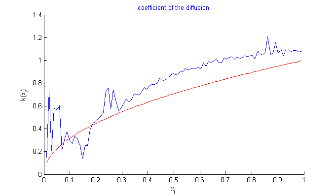
Figure 1. Graph of \(k\) in case \(\varepsilon=10^{-05}\)
In Table 1, the smallest value of \(J\) is reached when \(\varepsilon=10^{-05},\) and the Figure 1 shows that we can’t rebuild the coefficient \(k\) in case \(\varepsilon=10^{-05}\). We can conclude that the method of choosing \(\varepsilon\) by doing several tests for different epsilon values is not effective.
To overcome this problem, in case where \(k ^{b}\) is partially known, we propose in this work, a new approach based on Genetic Hybrid algorithms which consists to minimize the functional \(J\) without any regularization. This work is the continuity of [5] where the authors identify the initial state of a degenerate parabolic problem.
Firstly, with the aim of showing that the minimization problem and the direct problem are well-posed, we prove that the solution’s behavior changes continuously with respect to the initial conditions. Secondly, we show that the minimization problem has at least one minimum. Finally, The gradient of the cost function is computed using the adjoint state method. Also we present some numerical experiments to show the performance of this approach.
2. Well-posedness
Now we specify some notations we shall use. Let introduce the following functional spaces (see [6, 7, 8])
\begin{equation*} H^1_{\alpha,0}= \lbrace u\in H^1_{\alpha}\mid u(0)=u(1)=0 \rbrace, \end{equation*} \begin{equation*} H^1_{\alpha}= \lbrace {u\in L^2(\Omega)\cap H^1_{Loc}(]0,1])\mid x^{\frac{\alpha}{2}}u_x\in L^2(\Omega)} \rbrace. \end{equation*} With \begin{equation*} \parallel u\parallel ^2_{H^1_a(\Omega)}=\parallel u\parallel ^2_{L^2(\Omega)}+\parallel \sqrt{a} u_x\parallel ^2_{L^2(\Omega)}, \end{equation*} \begin{equation*} \parallel u\parallel^2_{H^2_a(\Omega)}=\parallel u\parallel ^2_{H^1_a(\Omega)}+\parallel (au_x)_x\parallel ^2_{L^2(\Omega)}, \end{equation*} \begin{equation*} < u,v >_{H^1_{\alpha}}=\int_{\Omega} (uv+ k(x)x^{\alpha}u_xv_x)\text{\ }dx. \end{equation*} We recall that (see [8] \(H^1_a\) is an Hilbert space and it is the closure of \(C^\infty_c(0,1)\) for the norm \(\parallel . \parallel_{H^1_a}.\) If \(\frac{1}{\sqrt{a}}\in L^1(\Omega)\) then the following injections \begin{equation*} H^1_a(\Omega)\hookrightarrow L^2(\Omega), \end{equation*} \begin{equation*} H^2_a(\Omega)\hookrightarrow H^1_a(\Omega), \end{equation*} \begin{equation*} H^1(0,T;L^2(\Omega))\cap L^2(0,T;D(A)) \hookrightarrow L^2(0,T;H^1_a)\cap C(0,T;L^2(\Omega)) \end{equation*} are compacts. Firstly, we prove that the problem (1) is well-posed, the functional \(J\) is continuous and G-derivable in \(A_{ad}\).
The weak formulation of the problem (1) is :
\begin{equation} \int_{\Omega}\partial_t u v \ dx+\int_{\Omega} \left(a(x)\partial_x u \partial_x v-\dfrac{\lambda }{x^{\beta }}u v\right) \ dx=\int_{\Omega}fv \ dx, \ \forall v \in H_0^1(\Omega). \end{equation}
Since \(a(x)=0\) at \(x=0\) and \(\displaystyle \underset{x \rightarrow 0}{\lim } \dfrac{\lambda }{x^{\beta }}= +\infty,\) the bilinear form \(\mathcal{B}\) is noncoercive and is non-continuous at \(x=0\). Consider the not bounded operator \((\mathcal{O},D(\mathcal{O}))\) where
\begin{equation} \mathcal{O}g=(k(x)x^{\alpha}g_x)_x+\frac{\lambda}{x^{\beta}}g, \ \forall g \in D(\mathcal{O}) \end{equation}
(11)
and \begin{equation*} D(\mathcal{O})=\lbrace {g\in H^1_{\alpha,0}\cap H^2_{Loc}(]0,1])\mid (x^{\alpha}g_x)_x+\frac{\lambda}{x^{\beta}}g\in L^2(\Omega)}\rbrace . \end{equation*} Let
\begin{equation} \displaystyle A_{ad} =\lbrace g\in H^1(\Omega); \Vert g\Vert_{H^1(\Omega)}\leq r \rbrace, \text{ where $r$ is a real strictly positive constant.} \end{equation}
(12)
We recall the following theorem
Theorem 2.1. (see [7, 10]) If \(f=0\) then for all \(u\in L^2(\Omega)\), the problem (1) has a unique weak solution
Theorem 2.2. (see [1]) For every \(u_0\in L^2(\Omega)\) and \(f\in L^2(Q_T),\) where \(Q_T=((0,T)\times\Omega)\) there exists a unique solution of problem (1). In particular, the operator \(\mathcal{O}: D(\mathcal{O})\longmapsto L^2(\Omega)\) is non positive and self-adjoint in \(L^2(\Omega)\) and it generates an analytic contraction semigroup of angle \(\pi/2.\) Moreover, let \(u_0\in D(\mathcal{O})\); then
\(f\in W^{1,1}(0,T;L^2(\Omega)\Rightarrow u\in C^0(0,T;D(\mathcal{O}))\cap C^1([0,T];L^2(\Omega)),\)
\(f\in L^2(L^2(Q_T))\Rightarrow u\in H^1(0,T;L^2(\Omega).\)
Theorem 2.3. Let \(u\) the weak solution of (1), the function
is continuous, and the functional \(J\) is continuous in \(A_{ad}\). Therefore, the problem 2 has at least one solution in \(A_{ad}\) .
Proof. [Proof of Theorem (2.3)] Let \(\delta k \in H^1(\Omega)\) a small variation such that \(k+\delta k \in A_{ad}\) and \(u_0\in D(\mathcal{O}).\) Consider \(\delta u =u ^{\delta }-u\), with \(u\) is the weak solution of (1) with diffusion coefficient \(k\), and \(u ^{\delta }\) is the weak solution of the following problem (17) with diffusion coefficient \(k^{\delta }=k+\delta k.\)
We have $$\int_{\Omega}\left((k+\delta k)x^{\alpha}(\partial_x \delta u)^2-\dfrac{\lambda }{x^{\beta }}(\delta u)^2 \right)dx\geq 0, $$ this implies that
\begin{equation} \int_{\Omega}\partial_t (\delta u)\delta udx-\int_{\Omega}\left(\delta k x^{\alpha}\partial_x u \right)_{x}\delta udx\leq 0 \end{equation}
(21)
and consequently
\begin{equation} \left |\int_{\Omega}\partial_t (\delta u)\delta udx \right |\leq \int_{\Omega}\left |\left(\delta k x^{\alpha}\partial_x u \right)_{x}\delta u \right |dx, \end{equation}
By integrating between \(0\) and \(t\) with \(t\in [0,T]\) we obtain
\begin{equation} \frac{1}{2}\Vert \delta u(t)\Vert_{L^2(\Omega)}^2\leq \left \| \delta k \right \|_{L^{\infty}(\Omega)}\int_{0}^{T}\int_{\Omega}\left | \partial_x u \partial_x\delta u\right |dxdt, \end{equation}
(24)
since \(u,\delta u\in H^1(0,T;L^2(\Omega)),\) we have \(\displaystyle\int_{0}^{T}\int_{\Omega} \left | \partial_x u \partial_x\delta u\right |dxdt< \infty\),
there is \(C>0,\) such that
\begin{equation} A_{ad} =\lbrace u\in H^1(\Omega); \Vert u\Vert_{H^1(\Omega)}\leq r \rbrace. \end{equation}
(27)
We have \(H^{1} (\Omega ) \underset{compact}{\hookrightarrow}L^{2}(\Omega ).\) Since the set \(A_{ad}\) is bounded in \(H^1(\Omega)\), then \(A_{ad}\) is a compact in \(L^{2}(\Omega ).\) Therefore, \(J\) has at least one minimum in \(A_{ad}\) Now we compute the gradient of \(J\) with the adjoint state method.
3. Gradient of \(J\)
We define the Gâteaux derivative of \(u\) at \(k\) in the direction \(h\in L^2( \Omega \times ] 0,T[)\), by
With \begin{equation*} t_j=j\Delta t, \quad j\in \{0,1,2,\dots,M+1\}, \end{equation*} where \(\Delta t\) is the step in time and \(T=(M+1)\Delta t\). The Gateaux derivative of \(J\) at \(k\) in the direction \(h\in L^2(\Omega)\) is given by \begin{equation*} \hat{J}(h)=\lim_{s \to 0} \frac{J(k+s h)-J(k)}{s }. \end{equation*} After some computations, we arrive at
Problem (32) is retrograde, we make the change of variable \(t\longleftrightarrow T-t\).
4. Numerical scheme
Step 1. Full discretization
Discrete approximations of these problems need to be made for numerical implementation. To resolve the direct problem and adjoint problem, we use the Method \(\theta\)-schema in time. This method is unconditionally stable for \(1 >\theta \geq \dfrac{1}{2}.\) Let \(h\) the steps in space and \(\Delta t\) the steps in time. Let \begin{equation*} x_{i}=ih, \ \ \ \ i\in \left\{ 0,1,2…N+1\right\}, \end{equation*} \begin{equation*} c(x_{i})=a(x_{i}), \end{equation*} \begin{equation*} t_{j}=j\Delta t, \ \ \ j\in \left\{0,1,2…M+1\right\}, \end{equation*} \begin{equation*} f_{i}^{j}=f(x_{i},t_{j}), \end{equation*} we put
We recall that the method of Thomas Simpson to calculate an integral is \begin{equation*} \displaystyle \int_a^b f(x) \ dx\simeq\frac{h}{2}\left[ f(x_0)+2 \sum_{i=1}^{\frac{N+1}{2}-1}f(x_{2i})+4 \sum_{i=1}^{\frac{N+1}{2}}f(x_{2i+1})+f(x_{N+1}) \right] \end{equation*} with \(x_0=a\), \(x_{N+1}=b\), \(x_i=a+ih\), \(i \ \in \left\lbrace 1..N+1\right\rbrace\). Let the function
The Genetic Algorithms (GA) are adaptive search and optimization methods that are based on the genetic processes of biological organisms. Their principles have been first laid down by Holland. The aim of GA is to optimize a problem-defined function, called the fitness function. To do this, GA maintain a population of individuals (suitably represented candidate solutions) and evolve this population over time. At each iteration, called generation, the new population is created by the process of selecting individuals according to their level of fitness in the problem domain and breeding them together using operators borrowed from natural genetics, as, for instance, crossover and mutation. As the population evolves, the individuals in general tend toward the optimal solution. The basic structure of a GA is the following: 1. Initialize a population of individuals; 2. Evaluate each individual in the population; 3. while termination criterion not reached do
{ 4. Select individuals for the next population; 5. Apply genetic operators (crossover, mutation) to produce new individuals; 6. Evaluate the new individuals;
} 7. return the best individual.
The hybrid methods combine principles from genetic algorithms and other optimization methods. In this approach, we will combine the genetic algorithm with method descent (steepest descent algorithm (FP)) as following:
We assume that we have a partial knowledge of background state \(k^b\) at certain points \((x_i)_{i\in I}\), \(I\subset \left\lbrace 1,2,..,N+1\right\rbrace\).
We assume the individual is a vector \(k\), the population is a set of individuals.
The initialization of individual is as following
\begin{equation}\label{EQCHOSEN} \begin{array}{l} \text{ for } i=1 \text{ to } N+1\\ \text{ if } i \in I \ k(x_i) \text{ is chosen in the vicinity of } k^b(x_i) \\ else \ k(x_i) \text{ is chosen randomly }\\ \text{end if }\\ \text{end for}\\ \end{array} \end{equation}
(49)
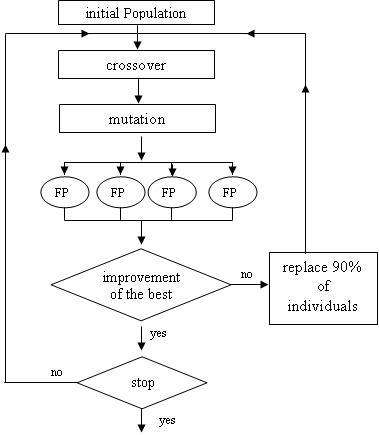
Starting by initial population, we apply genetic operators (crossover, mutation) to produce a new population in which each individual is an initial point for the descent method (FP). When a specific number of generations is reached without improvement of the best individual, only the fittest individuals (e.g. the first 10% fittest individuals in the population) survive. The remaining die and their place is occupied by new individuals with new genetic (45% are chosen randomly, the other 45% are chosen as (49)). At each generation we keep the best. The algorithm ends when \(\displaystyle \mid J(k)\mid < \mu \) or \(generation\geqslant Maxgen\), where \(\mu\) is a given precision (see Figure 2).
The main steps for descent method (FP) at each iteration are: – Calculate \(u^{j}\) solution of (1) with coefficient \(k^j\) – Calculate \(P^{j}\) solution of adjoint problem – Calculate the descent direction \(d_{j}=-\nabla J(k^j)\) – Find \(\displaystyle t_{j}=\underset{t>0}{argmin}\) \(J(k^j+td_{j})\) – Update the variable \(k^{j+1}=k^j+t_{j}d_{j}\).
The algorithm ends when \(\displaystyle \mid J(k^j)\mid< \mu\), where \(\mu\) is a given small precision. \(t_{j}\) is chosen by the inaccurate linear search by Rule Armijo-Goldstein as following: let \(\alpha_{i}, \beta \in [0,1[\) and \(\alpha>0\) if \(J(k^{j}+\alpha_i d_{j})\leqslant J(k^{j})+\beta \alpha_{i} d^{T}_{j}d_{j}\) \(t_{j}=\alpha_i\) and stop if not \(\alpha_i = \alpha \alpha_i\).
Figure 2. Hybrid Algorithm
6. Numerical experiments
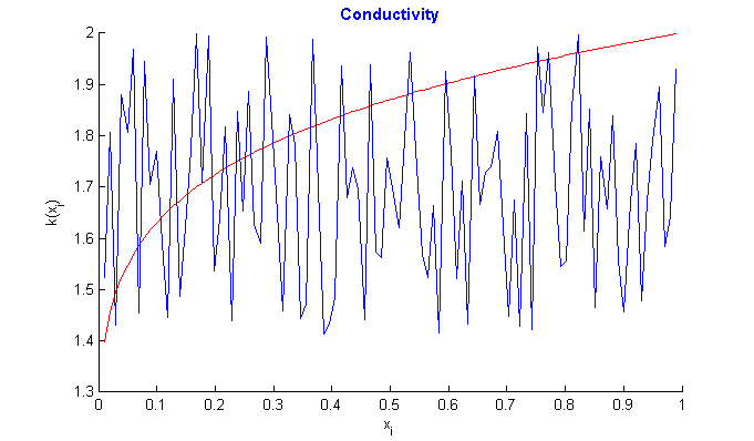
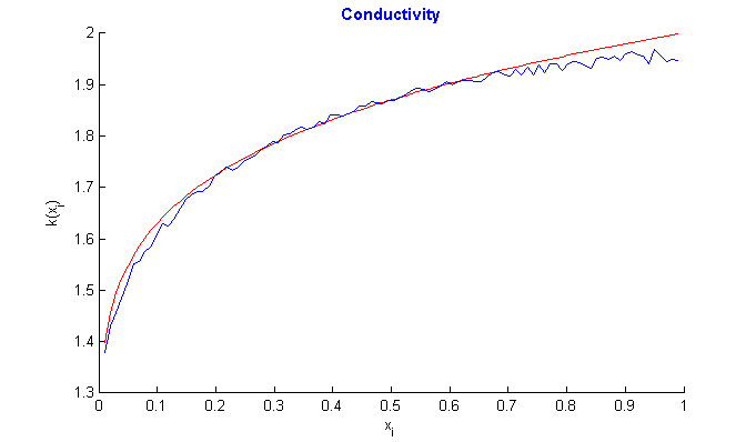
In this section, we do three tests: In the first test, we recall the result obtained by the algorithm of simple descent with \(\varepsilon=10^{-5}\) (Figure 1), In the second test, we turn only the genetic algorithm (Figure 2). Finally, in the third test, we turn test with hybrid approach with parameters \(\alpha=1/3,\)\(\beta=3/4\), \(\lambda=-2/3\), \(N=M=99,\) number of individuals \(=40\) , and number of generations \(=2000\). In the figures below, the exact function is drawn in red and rebuild function in blue.
Figure 3. Test with simple descent and \(\varepsilon=10^{-5}\).
Figure 4. Test with genetic algorithm.
Figure 5. Test with hybrid algorithm.
These tests show that we can’t rebuild the coefficient in the diffusion \(k\) by the descent method and genetic approach (Figure 3 and Figure 4), and the hybrid approach proves effective to reconstruct this coefficient (Figure 5).
7. Conclusion
We have presented in this paper a new approach based on a hybrid genetic algorithm for the determination of a coefficient in the diffusion term of some degenerate /singular one-dimensional linear parabolic equation from final data observations. Firstly, with the aim of showing that the minimization problem and the direct problem are well-posed, we have proved that the solution’s behavior changes continuously with respect to the initial conditions. Secondly, we have shown that the minimization problem has at least one minimum. Finally, we proved the differentiability of the cost function, which gives the existence of the gradient of this functional, that is computed using the adjoint state method. Also we have presented some numerical experiments to show the performance of this approach to construct the diffusion coefficient of a degenerate parabolic problem.
Competing Interests
The authors declares that he has no competing interests.
References
Vogel, C. R. (2002). Computational methods for inverse problems (Vol. 23). SIAM Frantiers in applied mathematics. [Google Scholor]
Engl, H. W., Hanke, M., & Neubauer, A. (1996). Regularization of inverse problems (Vol. 375). Springer Science & Business Media. [Google Scholor]
Hansen, P. C. (1992). Analysis of discrete ill-posed problems by means of the L-curve. SIAM review, 34(4), 561-580. [Google Scholor]
Tikhonov, A. N., Goncharsky, A., Stepanov, V. V., & Yagola, A. G. (2013). Numerical methods for the solution of ill-posed problems (Vol. 328). Springer Science & Business Media. [Google Scholor]
Atifi, K., Balouki, Y., Essoufi, E. H., & Khouiti, B. (2017). Identifying initial condition in degenerate parabolic equation with singular potential. International Journal of Differential Equations, 2017. [Google Scholor]
Alabau-Boussouira, F., Cannarsa, P., & Fragnelli, G. (2006). Carleman estimates for degenerate parabolic operators with applications to null controllability. Journal of Evolution Equations, 6(2), 161-204. [Google Scholor]
Hassi, E. M., Khodja, F. A., Hajjaj, A., & Maniar, L. (2013). Carleman estimates and null controllability of coupled degenerate systems. J. of Evol. Equ. and Control Theory, 2, 441-459. [Google Scholor]
Cannarsa, P., & Fragnelli, G. (2006). Null controllability of semilinear degenerate parabolic equations in bounded domains. Electronic Journal of Differential Equations (EJDE)[electronic only], 136, 1-20.[Google Scholor]
Emamirad, H., Goldstein, G., & Goldstein, J. (2012). Chaotic solution for the Black-Scholes equation. Proceedings of the American Mathematical Society, 140(6), 2043-2052.[Google Scholor]
Vancostenoble, J. (2011). Improved Hardy-Poincaré inequalities and sharp Carleman estimates for degenerate/singular parabolic problems. Discrete Contin. Dyn. Syst. Ser. S, 4(3), 761-790. [Google Scholor]
Hasanov, A., DuChateau, P., & Pektaş, B. (2006). An adjoint problem approach and coarse-fine mesh method for identification of the diffusion coefficient in a linear parabolic equation. Journal of Inverse and Ill-posed Problems jiip, 14(5), 435-463.[Google Scholor]