Open Journal of Mathematical Analysis

A new modified Adomian decomposition method for nonlinear partial differential equations

Djelloul Ziane, Rachid Belgacem\(^1\), Ahmed Bokhari
Laboratory of mathematics and its applications (LAMAP), University of Oran1 Ahmed Ben Bella, Oran, 31000, Algeria.; (D.Z)
Department of Physics, University of Hassiba Benbouali, Ouled Fares, Chlef 02180, Algeria.; (D.Z)
Department of Mathematics, University of Hassiba Benbouali, Ouled Fares, Chlef 02180, Algeria.; (R.B & A.B)
\(^1\)Corresponding Author: belgacemrachid02@yahoo.fr

Abstract

In literature, there are many methods for solving nonlinear partial differential equations. In this paper, we develop a new method by combining Adomian decomposition method and Shehu transform method for solving nonlinear partial differential equations. This method can be named as Shehu transform decomposition method (STDM). Some examples are solved to show that the STDM is easy to apply.

Keywords:

Adomian decomposition method, Shehu transform method, nonlinear partial differential equation.

1. Introduction

The use of integral transforms (Laplace, Sumudu, Natural, Elzaki, Aboodh, Shehu and other transforms) in solving linear differential equations as well as integral equations has developed significantly as a result of the advantages of these transformations. Through these transforms, many problems of engineering and sciences have been solved. However, it was found that these transforms remain limited in solving equations that contain a nonlinear part.

To take advantage of these transformations and to use them to solve nonlinear differential equations, researchers in the field of mathematics were guided to the idea of their composition with some methods such as: Adomian decomposition method (ADM) [1, 2, 3, 4], homotopy analysis method [5, 6, 7, 8], variational iteration method (VIM) [9, 10, 11,12], homotopy perturbation method (HPM) [13, 14, 15,16] and DJ iteration method [17, 18, 19, 20].

The objective of the present study is to combine two powerful methods, Adomian decomposition method and Shehu transform method to get a better method to solve nonlinear partial differential equations. The modified method is called Shehu transform decomposition method (STDM). We apply our modified method to solve some examples of nonlinear partial differential equations.

2. Basics of Shehu transform

In this section we define Shehu transform and gave its important properties [21].

Definition

The Shehu transform of the function \(v(t)\) of exponential order is defined over the set of functions:

\begin{equation} A=\left\{ v(t):\exists N,\text{ }k_{1},k_{2}>0,\text{ }\left\vert v(t)\right\vert < N\exp \left( \frac{\left\vert t\right\vert }{k_{i}}\right) , \text{ }if\text{ }t\in (-1)^{j}\times \lbrack 0,\text{ }\infty )\right\} , \label{AA1} \end{equation}
(1)
by the following integral
\begin{eqnarray} \hat{S}\left[ v(t)\right] &=&\left[ V(s,u)\right] =\int\limits_{0}^{\infty }\exp (\frac{-st}{u})v(t)dt \notag \\ &=&\lim_{\alpha \longrightarrow \infty }\int\limits_{0}^{\alpha }\exp (\frac{ -st}{u})v(t)dt,\text{ }s>0,u>0. \label{A2} \end{eqnarray}
(2)
It converges if the limit of the integral exists, and diverges if not.

The inverse Shehu transform is given as:

\begin{equation} \hat{S}^{-1}\left[ V(s,u)\right] =v(t), \text{ for }t\geqslant 0. \label{A3} \end{equation}
(3)
Equivalently
\begin{equation} v(t)=\ \hat{S}^{-1}\left[ V(s,u)\right] =\frac{1}{2\pi i}\int\limits_{\alpha -i\infty }^{\alpha +i\infty }\frac{1}{u}\exp (\frac{st}{u})V(s,u)ds, \label{A4} \end{equation}
(4)
where \(s\) and \(u\) are the Shehu transform variables, and \(\alpha \) is a real constant and the integral in Equation (4) is taken along \(s=\alpha \) in the complex plane \(s=x+iy.\)

Theorem 2. (The sufficient condition for the existence of Shehu transform [21]. If the function \(v(t)\) is piecewise continues in every finite interval \(0\leqslant t\leqslant \beta \) and of exponential order \(\alpha \) for \(t>\beta \). Then its Shehu transform \(V(s;u)\) exists.

Theorem 3. (Derivative of Shehu transform [21]. If the function \(v^{\left( n\right) }(t)\) is the \(n\)th derivative of the function \(v(t)\in A\) with respect to \( ^{\prime }t^{\prime }\) then its Shehu transform is defined as:

\begin{equation} \hat{S}\left[ v^{\left( n\right) }(t)\right] =\frac{s^{n}}{u^{n}} V(s,u)-\sum\limits_{n=0}^{\infty }\left( \frac{s}{u}\right) ^{n-(k+1)}v^{\left( k\right) }(0). \label{A5} \end{equation}
(5)
Taking \(n=1,2\) and \(3\) in Equation (5), we obtain the following derivatives with respect to \(t\):
\begin{equation} \hat{S}\left[ v^{\prime }(t)\right] =\frac{s}{u}V(s,u)-v(0). \label{A6} \end{equation}
(6)
\begin{equation} \hat{S}\left[ v^{\prime \prime }(t)\right] =\frac{s^{2}}{u^{2}}V(s,u)-\frac{s }{u}v(0)-v^{\prime }(0). \label{A7} \end{equation}
(7)
\begin{equation} \hat{S}\left[ v^{\prime \prime \prime }(t)\right] =\frac{s^{3}}{u^{3}}V(s,u)- \frac{s^{2}}{u^{2}}v(0)-\frac{s}{u}v^{\prime }(0)-v^{\prime \prime }(0). \label{A8} \end{equation}
(8)
Now, we summarize some important properties of this transform [21].
  1. Linearity: \(\hat{S}\left[ (\alpha f(t)+\beta g(t)\right] =\alpha \hat{S}\left[ f(t)\right] +\alpha \hat{S}\left[ g(t)\right] .\)
  2. Change of scale: \(\hat{S}\left[ f(\beta t)\right] =\frac{u}{ \beta }V\left( \frac{s}{\beta },u\right) .\)
Other properties are given in the Table 1.
Table 1. Some important properties of Shehu transform.
\(v(t)\) \(\hat{S}\left[ v(t)\right]\) \(v(t)\) \(\hat{S}\left[ v(t)\right]\)
\(1\) \(\frac{u}{s}\) \(\sin at\) \(\frac{au^{2}}{s^{2}+a^{2}u^{2}}\)
\(t\) \(\frac{u^{2}}{s^{2}}\) \(\cos at\) \(\frac{us}{s^{2}+a^{2}u^{2}}\)
\(\frac{t^{n}}{n!},\) \(n=0,1,2,..\) \(\left( \frac{u}{s}\right)^{n+1}\) \(\sinh at\) \(\frac{au^{2}}{s^{2}-a^{2}u^{2}}\)
\(\frac{t^{n}\exp (at)}{n!}\) \(\frac{u^{n+1}}{\left(s-au\right) ^{n+1}}\) \(\cosh at\) \(\frac{us}{s^{2}-a^{2}u^{2}}\)

Proposition 4. If \(\frac{\partial v(x,t)}{\partial t}\) and \(\frac{\partial ^{2}v(x,t)}{ \partial t^{2}}\) exist, then

\begin{equation} \hat{S}\left[ \frac{\partial v(x,t)}{\partial t}\right] =\frac{s}{u} V(x,s,u)-v(x,0). \label{A9} \end{equation}
(9)
\begin{equation} \hat{S}\left[ \frac{\partial ^{2}v(x,t)}{\partial t^{2}}\right] =\frac{s^{2} }{u^{2}}V(x,s,u)-\frac{s}{u}v(x,0)-\frac{\partial v(x,0)}{\partial t}. \label{A10} \end{equation}
(10)

Proof. By means of integration by parts, we get \begin{eqnarray*} \hat{S}\left[ \frac{\partial v(x,t)}{\partial t}\right] &=&\int\limits_{0}^{ \infty }e^{\frac{-st}{u}}\frac{\partial v(x,t)}{\partial t}dt=\lim_{\tau \longrightarrow \infty }\int\limits_{0}^{\tau }e^{\frac{-st}{u}}\frac{ \partial v(x,t)}{\partial t}dt \\ &=&\lim_{\tau \longrightarrow \infty }\left( \left[ v(x,t)e^{\frac{-st}{u}} \right] _{0}^{\tau }+\frac{s}{u}\int\limits_{0}^{\tau }e^{\frac{-st}{u} }v(x,t)dt\right) \\ &=&\frac{s}{u}V(x,s,u)-v(x,0). \end{eqnarray*} Let \(\frac{\partial v(x,t)}{\partial t}=w(x,t)\), then, by using Equation (2) and Equation (9), we get: \ \ \begin{eqnarray*} \hat{S}\left[ \frac{\partial ^{2}v(x,t)}{\partial t^{2}}\right] &=&\hat{S} \left[ \frac{\partial w(x,t)}{\partial t}\right] =\frac{s}{u}\hat{S}\left[ w(x,t)\right] -w(x,0) \\ &=&\frac{s}{u}\hat{S}\left[ \frac{\partial v(x,t)}{\partial t}\right] -\frac{ \partial v(x,0)}{\partial t} \\ &=&\frac{s^{2}}{u^{2}}V(x,s,u)-\frac{s}{u}v(x,0)-\frac{\partial v(x,0)}{ \partial t}. \end{eqnarray*}

Proposition 5. Let \(V(x,s,u)\) is the Shehu transform of \(v(x,t),\) then

\begin{equation} \hat{S}\left[ \frac{\partial ^{n}v(x,t)}{\partial t^{n}}\right] =\frac{s^{n} }{u^{n}}V(x,s,u)-\sum\limits_{k=0}^{n-1}\left( \frac{s}{u}\right) ^{n-(k+1)} \frac{\partial ^{k}v(x,0)}{\partial t^{k}}. \label{A11} \end{equation}
(11)

Proof. We use use mathematical induction to prove (11). By means of Equation (9), the formula (11) is true for \(n=1\) and suppose

\begin{equation} \hat{S}\left[ \frac{\partial ^{n}v(x,t)}{\partial t^{n}}\right] =\frac{s^{n} }{u^{n}}V(x,s,u)-\sum\limits_{k=0}^{n-1}\left( \frac{s}{u}\right) ^{n-(k+1)} \frac{\partial ^{k}v(x,0)}{\partial t^{k}}, \label{A13} \end{equation}
(12)
Let \(\frac{\partial ^{n}v(x,t)}{ \partial t^{n}}=w(x,t)\) and using (9) and (12), we have: \begin{eqnarray*} \ \ \hat{S}\left[ \frac{\partial ^{n+1}v(x,t)}{\partial t^{n+1}}\right] &=& \hat{S}\left[ \frac{\partial w(x,t)}{\partial t}\right] =\frac{s}{u}\hat{S} \left( w(x,t)\right) -w(x,0) \\ &=&\frac{s}{u}\left[ \frac{s^{n}}{u^{n}}V(x,s,u)-\sum_{k=0}^{n-1} \left( \frac{s}{u}\right) ^{n-(k+1)}\frac{\partial ^{k}v(x,0)}{\partial t^{k} }\right] -\frac{\partial ^{n}v(x,0)}{\partial t^{n}} \\ &=&\frac{s^{n+1}}{u^{n+1}}V(x,s,u)-\sum_{k=0}^{n-1}\left( \frac{s}{u} \right) ^{n+1-(k+1)}\frac{\partial ^{k}v(x,0)}{\partial t^{k}}-\frac{ \partial ^{n}v(x,0)}{\partial t^{n}} \\ &=&\frac{s^{n+1}}{u^{n+1}}V(x,s,u)-\sum_{k=0}^{n}\left( \frac{s}{u} \right) ^{n+1-(k+1)}\frac{\partial ^{k}v(x,0)}{\partial t^{k}}. \end{eqnarray*}

3. Main results

3.1. Shehu transform decomposition method

To illustrate the basic idea of this method, we consider a general nonlinear nonhomogeneous partial differential equation
\begin{equation} \ \frac{\partial ^{m}U(x,t)}{\partial t^{m}}+RU(x,t)+NU(x,t)=g(x,t), \label{C1} \end{equation}
(13)
where \(\frac{\partial ^{m}U(x,t)}{\partial t^{m}}\) is the partial derivative of the function \(U(x,t)\) of order \(m\) \((m=1,2,3)\), \(R\) is the linear differential operator, \(N\) represents the general nonlinear differential operator, and \(g(x,t)\) is the source term. Applying the Shehu transform (denoted in this paper by \(\hat{S}\)) on both sides of Equation (13), we get
\begin{equation} \ \hat{S}\left[ \ \frac{\partial ^{m}U(x,t)}{\partial t^{m}}\right] +\hat{S} \left[ RU(x,t)+NU(x,t)\right] =\hat{S}\left[ g(x,t)\right] . \label{C3} \end{equation}
(14)
Using the properties of Shehu transform, we obtain
\begin{equation} \frac{s^{m}}{u^{m}}\hat{S}\left[ U(x,t)\right] =\sum\limits_{k=0}^{m-1} \left( \frac{s}{u}\right) ^{m-(k+1)}\frac{\partial ^{k}U(x,0)}{\partial t^{k} }+\hat{S}\left[ g(x,t)\right] -\hat{S}\left[ RU(x,t)+NU(x,t)\right] , \label{C4} \end{equation}
(15)
where \(m=1,2,3.\) Thus, we have
\begin{equation} \hat{S}\left[ U(x,t)\right] =\sum\limits_{k=0}^{m-1}\left( \frac{u}{s} \right) ^{k+1}\frac{\partial ^{k}U(x,0)}{\partial t^{k}}+\frac{u^{m}}{s^{m}} \hat{S}\left[ g(x,t)\right] -\frac{u^{m}}{s^{m}}\hat{S}\left[ RU(x,t)+NU(x,t) \right] . \label{C5} \end{equation}
(16)
Operating the inverse transform on both sides of Equation (16), we get
\begin{equation} U(x,t)=G(x,t)-\hat{S}^{-1}\left( \frac{u^{m}}{s^{m}}\hat{S}\left[ RU(x,t)+NU(x,t)\right] \right) , \label{C6} \end{equation}
(17)
where \(G(x,t)\), represents the term arising from the source term and the prescribed initial conditions. The second step in Shehu transform decomposition method, is that we represent the solution as an infinite series given below
\begin{equation} U(x,t)=\sum\limits_{n=0}^{\infty }U_{n}(x,t), \label{C7} \end{equation}
(18)
and the nonlinear term can be decomposed as:
\begin{equation} \ NU(x,t)=\sum\limits_{n=0}^{\infty }A(U), \label{C8} \end{equation}
(19)
where \(A_{n}\) are Adomian polynomials [22] of \( U_{0},U_{1},U_{2},...,U_{n}\) and it can be calculated by the formula:\(\ \ \)
\begin{equation} \ A_{n}=\frac{1}{n!}\frac{\partial ^{n}}{\partial \lambda ^{n}}\left[ N\left( \sum\limits_{i=0}^{\infty }\lambda ^{i}U_{i}\right) \right] _{\lambda =0},\ \ n=0,1,2,\cdots . \label{C9} \end{equation}
(20)
Substituting (18) and (19) in (17), we have
\begin{equation} \sum\limits_{n=0}^{\infty }U_{n}(x,t)=G(x,t)-\hat{S}^{-1}\left[ \frac{u^{m}}{ s^{m}}\hat{S}\left[ R\sum\limits_{n=0}^{\infty }U_{n}(x,t)+\sum\limits_{n=0}^{\infty }A_{n}(U)\right] \right] . \label{C10} \end{equation}
(21)
On comparing both sides of the Equation (21), we get
\begin{equation} \begin{array}{c} \ U_{0}(x,t)=G(x,t), \\ \ U_{1}(x,t)=-\hat{S}^{-1}\left[ \frac{u^{m}}{s^{m}}\hat{S}\left[ RU_{0}(x,t)+A_{0}(U)\right] \right] , \\ U_{2}(x,t)=-\hat{S}^{-1}\left[ \frac{u^{m}}{s^{m}}\hat{S}\left[ RU_{1}(x,t)+A_{1}(U)\right] \right] , \\ U_{3}(x,t)=-\hat{S}^{-1}\left[ \frac{u^{m}}{s^{m}}\hat{S}\left[ RU_{2}(x,t)+A_{2}(U)\right] \right] , \\ \vdots \end{array} \label{C11} \end{equation}
(22)
In general, the recursive relation is given as:
\begin{equation} U_{n+1}(x,t)=-\hat{S}^{-1}\left[ \frac{u^{m}}{s^{m}}\hat{S}\left[ RU_{n}(x,t)+A_{n}(U)\right] \right] , \label{C12} \end{equation}
(23)
where \(m=1,2,3,\) and \(n\geqslant 0.\) Finally, we approximate the analytical solution \(U(x,t)\) by:
\begin{equation} U(x,t)=\lim_{N\rightarrow \infty }\sum\limits_{n=0}^{N}U_{n}(x,t), \label{C13} \end{equation}
(24)
The above series solutions generally converge very rapidly [23].

3.2. Application

Here, we apply Shehu transform decomposition method to solve some nonlinear partial differential equations.

Example 1. Consider the nonlinear KdV equation [24]:

\begin{equation} \ \ U_{t}+UU_{x}-U_{xx}=0, \label{C14} \end{equation}
(25)
with the initial condition:
\begin{equation} \ U(x,0)=x. \label{C15} \end{equation}
(26)
Applying the Shehu transform on both sides of Equation (25), we get
\begin{equation} \hat{S}\left[ \ U_{t}\right] +\hat{S}\left[ UU_{x}\right] -\hat{S}\left[ U_{xx}\right] =0. \label{C16} \end{equation}
(27)
By means of the properties of Shehu transform, we get
\begin{equation} \hat{S}\left[ \ U(x,t)\right] =x-\frac{u}{s}E\left[ UU_{x}-U_{xx}\right] . \label{C17} \end{equation}
(28)
Taking the inverse Shehu transform on both sides of Equation (28), we obtain
\begin{equation} U(x,t)=x-\hat{S}^{-1}\left( \frac{u}{s}\hat{S}\left[ UU_{x}-U_{xx}\right] \right) . \label{C18} \end{equation}
(29)
By applying the aforesaid decomposition method, we have
\begin{equation} \ \sum\limits_{n=0}^{\infty }U(x,t)=x-\hat{S}^{-1}\left[ \frac{u}{s}\hat{S} \left( \sum\limits_{n=0}^{\infty }A_{n}(U)-\sum\limits_{n=0}^{\infty }(U_{n})_{xx}\right) \right] \label{C19} \end{equation}
(30)
On comparing both sides of Equation (30), we get
\begin{equation} \begin{array}{c} \ U_{0}(x,t)=x, \\ \ U_{1}(x,t)=-\hat{S}^{-1}\left[ \frac{u}{s}\hat{S}\left( A_{0}(U)-U_{0xx}(x,t)\right) \right] , \\ U_{2}(x,t)=-\hat{S}^{-1}\left[ \frac{u}{s}\hat{S}\left( A_{1}(U)-U_{1xx}(x,t)\right) \right] , \\ U_{3}(x,t)=-\hat{S}^{-1}\left[ \frac{u}{s}\hat{S}\left( A_{2}(U)-U_{2xx}(x,t)\right) \right] , \\ \vdots \end{array} \label{C20} \end{equation}
(31)
The first few components of \(A_{n}(U)\) polynomials [22], for example, are given by:
\begin{equation} \begin{array}{c} A_{0}(U)=U_{0}U_{0,x}, \\ A_{1}(U)=U_{0}U_{1,x}+U_{1}U_{0,x}, \\ A_{2}(U)=U_{0}U_{2,x}+U_{2}U_{0,x}+U_{1}U_{1,x}, \\ \vdots \end{array} \label{C21} \end{equation}
(32)
Using the iteration formulas (31) and the Adomian polynomials (32), we obtain
\begin{equation} \ \begin{array}{c} \ U_{0}(x,t)=x, \\ U_{1}(x,t)=-xt, \\ U_{2}(x,t)=xt^{2}, \\ U_{3}(x,t)=-xt^{3}, \\ \vdots \end{array} \label{C22} \end{equation}
(33)
Based on the formula (24), we get
\begin{equation} U(x,t)=x-xt+xt^{2}-xt^{3}+\cdots, \label{C23} \end{equation}
(34)
which gives
\begin{equation} U(x,t)=\frac{x}{1+t},\ \ \ \left\vert t\right\vert < 1, \label{C24} \end{equation}
(35)
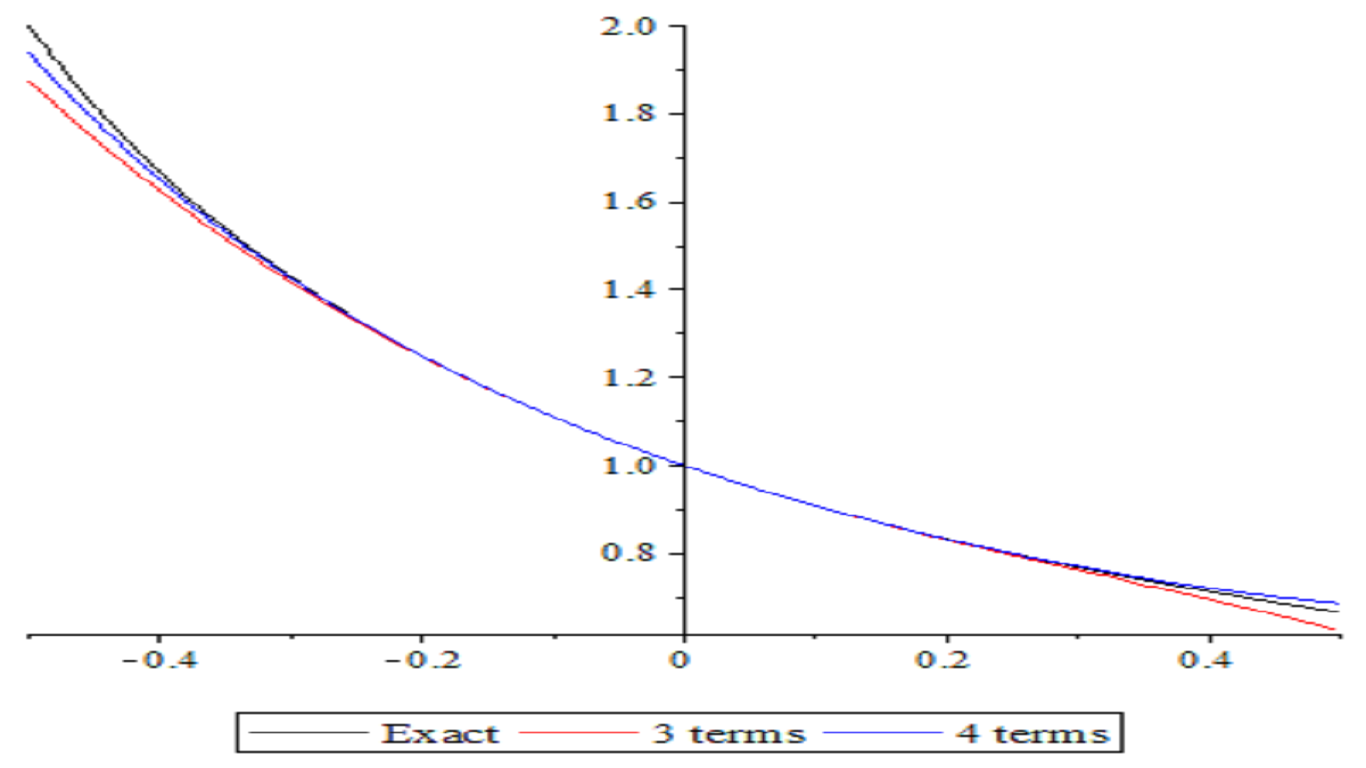
which is an exact solution to the KdV equation as presented in [25]. The graphs of exact solution and approximate solutions of Equation (25) for 3 terms and 4 terms is given in Figure 1.

Figure 1. The graphs of exact solution and approximate solutions of Equation (25) for 3 terms and 4 terms.

Example 2. Consider the nonlinear gas dynamics equation:

\begin{equation} U_{t}+UU_{x}-U(1-U)=0,t>0, \label{Z1} \end{equation}
(36)
with the initial condition:\(\ \)
\begin{equation} U(x,0)=e^{-x}.\ \ \label{Z2} \end{equation}
(37)
Applying the Shehu transform and its inverse on both sides of Equation (36), we get
\begin{equation} U(x,t)=e^{-x}-\hat{S}^{-1}[\frac{u}{s}\hat{S}\left( UU_{x}+U^{2}-U\right) ]. \label{Z3} \end{equation}
(38)
By applying the aforesaid Decomposition Method, we have
\begin{equation} \sum\limits_{n=0}^{\infty }U_{n}(x,y)=e^{-x}-\hat{S}^{-1}\left[ \frac{u}{s} \hat{S}\left( \sum\limits_{n=0}^{\infty }A_{n}(U)+\sum\limits_{n=0}^{\infty }B_{n}(U)-\sum\limits_{n=0}^{\infty }U_{n}\right) \right] . \label{Z4} \end{equation}
(39)
On comparing both sides of Equation (39), we obtain
\begin{equation} \begin{array}{c} \ U_{0}(x,t)=e^{-x}, \\ \ U_{1}(x,t)=-\hat{S}^{-1}\left[ \frac{u}{s}\hat{S}\left( A_{0}(U)+B_{0}(U)-U_{0}(x,t)\right) \right] , \\ U_{2}(x,t)=-\hat{S}^{-1}\left[ \frac{u}{s}\hat{S}\left( A_{1}(U)+B_{0}(U)-U_{1}(x,t)\right) \right] , \\ U_{3}(x,t)=-\hat{S}^{-1}\left[ \frac{u}{s}\hat{S}\left( A_{2}(U)+B_{0}(U)-U_{2}(x,t)\right) \right] , \\ \vdots \end{array} \label{Z5} \end{equation}
(40)
The first few components of \(A_{n}(U)\) polynomials [2] is given by (32), and for \(B_{n}(U)\) for example, given as follows:
\begin{equation} \begin{array}{c} B_{0}(U)=U_{0}U_{0}, \\ B_{1}(U)=2U_{0}U_{1}, \\ B_{2}(U)=2U_{0}U_{2}+U_{1}^{2}, \\ \vdots \end{array} \label{Z6} \end{equation}
(41)
Using the iteration formulas (40) and the Adomian polynomials (32), (41), we get the first terms of the solution series that is given by:
\begin{equation} \ \begin{array}{c} \ U_{0}(x,t)=e^{-\varkappa }, \\ U_{1}(x,t)=e^{-\varkappa }t, \\ U_{2}(x,t)=e^{-\varkappa }\frac{t^{2}}{2!}, \\ U_{3}(x,t)=e^{-\varkappa }\frac{t^{3}}{3!}, \\ \vdots \end{array} \label{Z7} \end{equation}
(42)
So, the approximate series solution of Equation (36) is given as:
\begin{equation} U(x,t)=e^{-x}\left[ 1+t+\frac{t^{2}}{2!}+\frac{t^{3}}{3!}+\cdots \right] . \label{Z28} \end{equation}
(43)
And in the closed form, is given by:
\begin{equation} U(x,t)=e^{-x}e^{t}=e^{t-x}. \label{Z29} \end{equation}
(44)
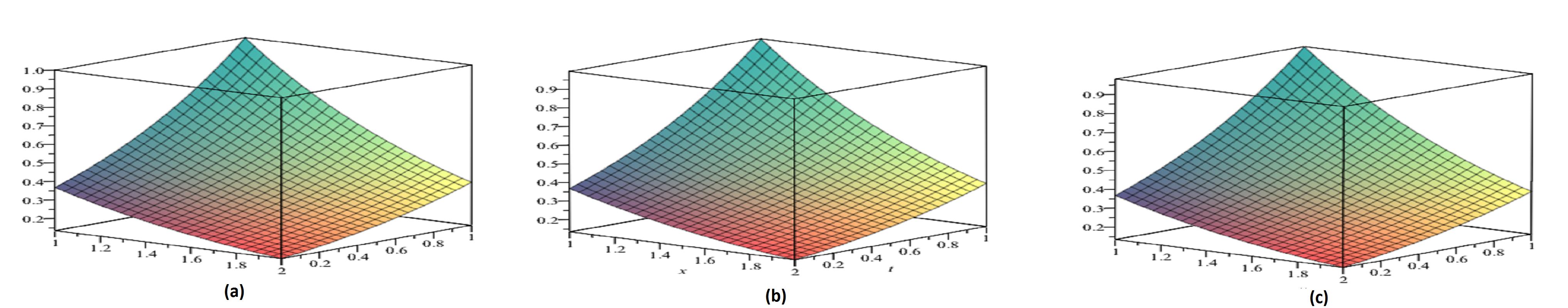
This result is the same as that obtained in [26] using homotopy analysis method. In Figure 2, \((a)\) represents the graph of exact solution, \((b)\) represents the graph of approximate solutions in 5 terms and \((c)\) represents the graph of approximate solutions in 4 terms.

Figure 2. \((a)\) Represents the graph of exact solution, \((b)\) represents the graph of approximate solutions in 5 terms, \((c)\) represents the graph of approximate solutions in 4 terms.

Example 3. Consider the nonlinear wave-like equation with variable coefficients:

\begin{equation} \ U_{tt}=x^{2}\frac{\partial }{\partial x}\left( U_{x}U_{xx}\right) -x^{2}\left( U_{xx}\right) ^{2}-U,\text{ }0< x< 1,\text{ }t>0, \label{T25} \end{equation}
(45)
with\ the initial conditions:
\begin{equation} \ U(x,0)=0,\text{ }U_{t}(x,0)=x^{2}. \label{T26} \end{equation}
(46)
Applying the Shehu transform and its inverse on both sides of Equation (45), we get
\begin{equation} U(x,t)=x^{2}t+\hat{S}^{-1}\left[ \frac{u^{2}}{s^{2}}\hat{S}\left( x^{2}\frac{ \partial }{\partial x}\left( U_{x}U_{xx}\right) -x^{2}\left( U_{xx}\right) ^{2}-U\right) \right] . \label{T30} \end{equation}
(47)
By applying the aforesaid Decomposition Method, we have
\begin{equation} \sum\limits_{n=0}^{\infty }U(x,t)=x^{2}t+\hat{S}^{-1}\left[ \frac{u^{2}}{ s^{2}}\hat{S}\left( x^{2}\frac{\partial }{\partial x}\left( \sum\limits_{n=0}^{\infty }C_{n}(U)\right) -x^{2}\sum\limits_{n=0}^{\infty }D_{n}(U)-\sum\limits_{n=0}^{\infty }U_{n}\right) \right] . \label{T31} \end{equation}
(48)
Comparing both sides of Equation (48), we obtain
\begin{equation} \begin{array}{c} U_{0}(x,t)=x^{2}t, \\ U_{1}(x,t)=\hat{S}^{-1}\left[ \frac{u^{2}}{s^{2}}\hat{S}\left( x^{2}\frac{ \partial }{\partial x}\left( C_{0}(U)\right) -x^{2}D_{0}(U)-U_{0}\right) \right] , \\ U_{2}(x,t)=\hat{S}^{-1}\left[ \frac{u^{2}}{s^{2}}\hat{S}\left( x^{2}\frac{ \partial }{\partial x}\left( C_{1}(U)\right) -x^{2}D_{1}(U)-U_{1}\right) \right] , \\ U_{3}(x,t)=\hat{S}^{-1}\left[ \frac{u^{2}}{s^{2}}\hat{S}\left( x^{2}\frac{ \partial }{\partial x}\left( C_{2}(U)\right) -x^{2}D_{2}(U)-U_{2}\right) \right] \\ \vdots \end{array} \label{T32} \end{equation}
(49)
The first few components of \(C_{n}(U)\) and \(D_{n}(U)\) Adomian polynomials [22], for example, are given by:
\begin{equation} \begin{array}{c} C_{0}(U)=U_{0,x}U_{0,xx}, \\ C_{1}(U)=U_{0,x}U_{1,xx}+U_{1,x}U_{0,xx}, \\ C_{2}(U)=U_{0,x}U_{2,xx}+U_{2,x}U_{0,xx}+U_{1,x}U_{1,xx}, \\ \vdots \end{array} \label{T33} \end{equation}
(50)
and
\begin{equation} \begin{array}{c} D_{0}(U)=\left( U_{0,xx}\right) ^{2}, \\ D_{1}(U)=2U_{0,xx}U_{1,xx}, \\ D_{2}(U)=2U_{0,xx}U_{2,xx}+\left( U_{1,xx}\right) ^{2}, \\ \vdots \end{array} \label{T34} \end{equation}
(51)
Using the iteration formulas (49) and the Adomian polynomials (50) and (51), we obtain
\begin{equation} \begin{array}{c} U_{0}(x,t)=x^{2}t, \\ U_{1}(x,t)=-x^{2}\frac{t^{3}}{3!}, \\ U_{2}(x,t)=x^{2}\frac{t^{5}}{5!}, \\ U_{3}(x,t)=-x^{2}\frac{t^{7}}{7!}, \\ \vdots \end{array} \label{T35} \end{equation}
(52)
The first terms of the approximate solution of Equation (45), is given by
\begin{equation} U(x,t)=x^{2}\left[ t-\frac{t^{3}}{3!}+\frac{t^{5}}{5!}-\frac{t^{7}}{7!} +\cdots \right] . \label{T36} \end{equation}
(53)
And in the closed form:
\begin{equation} U(x,t)=x^{2}\sin (t). \label{T37} \end{equation}
(54)
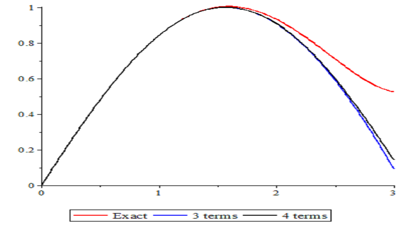
This result represents the exact solution of the Equation (45) as presented in [27] The graphs of exact solution and approximate solutions of Equation (45) for 3 terms and 4 terms are shown in Figure 3.

Figure 3. The graphs of exact solution and approximate solutions of Equation (45) for 3 terms and 4 terms.

4. Conclusion

The coupling of Adomian decomposition method (ADM) and Shehu transform method proved very effective to solve nonlinear partial differential equations. We can say that this method is easy to implement and is very effective, as it allows us to know the exact solution after calculate the first three terms only. As a result, the conclusion that comes through this work is that (STDM) can be applied to other nonlinear partial differential equations of higher order, due to the efficiency and flexibility.

Author Contributions

All authors contributed equally to the writing of this paper. All authors read and approved the final manuscript.

Competing Interests

The author(s) do not have any competing interests in the manuscript.

References

  1. Adomian, G., & Rach, R. (1990). Equality of partial solutions in the decomposition method for linear or nonlinear partial differential equations. Computers & Mathematics with Applications, 19(12), 9-12. [Google Scholor]
  2. Adomian, G. (2013). Solving frontier problems of physics: the decomposition method (Vol. 60). Springer Science & Business Media. [Google Scholor]
  3. Adomian, G. (1994). Solution of physical problems by decomposition. Computers & Mathematics with Applications, 27(9-10), 145-154.[Google Scholor]
  4. Adomian, G. (1998). Solutions of nonlinear PDE. Applied Mathematics Letters, 11(3), 121-123. [Google Scholor]
  5. Liao, S. J. (1992). The proposed homotopy analysis technique for the solution of nonlinear problems (Doctoral dissertation, Ph. D. Thesis, Shanghai Jiao Tong University). [Google Scholor]
  6. Raton, B. (2003). Beyond Perturbation: Introduction to Homotopy Analysis Method. Chapman and Hall/CRC Press, Boca Raton. [Google Scholor]
  7. Liao, S. (2004). On the homotopy analysis method for nonlinear problems. Applied Mathematics and Computation, 147(2), 499-513. [Google Scholor]
  8. Liao, S. (2009). Notes on the homotopy analysis method: some definitions and theorems. Communications in Nonlinear Science and Numerical Simulation, 14(4), 983-997. [Google Scholor]
  9. He, J. (1997). A new approach to nonlinear partial differential equations. Communications in Nonlinear Science and Numerical Simulation, 2(4), 230-235. [Google Scholor]
  10. He, J. H. (1998). Approximate analytical solution for seepage flow with fractional derivatives in porous media. Computer Methods in Applied Mechanics and Engineering, 167(1-2), 57-68. [Google Scholor]
  11. He, J. H. (1998). A variational iteration approach to nonlinear problems and its applications. Mech. Appl, 20(1), 30-31. [Google Scholor]
  12. He, J. H., & Wu, X. H. (2007). Variational iteration method: new development and applications. Computers & Mathematics with Applications, 54(7-8), 881-894. [Google Scholor]
  13. He, J. H. (1999). Homotopy perturbation technique. Computer methods in applied mechanics and engineering, 178(3-4), 257-262. [Google Scholor]
  14. He, J. H. (2005). Application of homotopy perturbation method to nonlinear wave equations. Chaos, Solitons & Fractals, 26(3), 695-700. [Google Scholor]
  15. He, J. H. (2000). A coupling method of homotopy technique and perturbation to Volterra’s integro-differential equation. International Journal of Non-Linear Mechanics, 35(1), 37-43. [Google Scholor]
  16. He, J. H. (2000). A new perturbation technique which is also valid for large parameters. Journal of Sound and Vibration, 5(229), 1257-1263.[Google Scholor]
  17. Daftardar-Gejji, V., & Jafari, H. (2006). An iterative method for solving nonlinear functional equations. Journal of Mathematical Analysis and Applications, 316(2), 753-763. [Google Scholor]
  18. Hemeda, A. A. (2012). New iterative method: application to nth-order integro-differential equations. In International Mathematical Forum (Vol. 7, No. 47, pp. 2317-2332). [Google Scholor]
  19. AL-Jawary, M. A. (2014). A reliable iterative method for Cauchy problems. Mathematical Theory and Modeling, 4, 148-153. [Google Scholor]
  20. Patade, J., & Bhalekar, S. (2015). Approximate analytical solutions of Newell-Whitehead-Segel equation using a new iterative method. World Journal of Modelling and Simulation, 11(2), 94-103. [Google Scholor]
  21. Maitama, S., & Zhao, W. (2019). New integral transform: Shehu transform a generalization of Sumudu and Laplace transform for solving differential equations. International Journal of Nonlinear Analysis and Applications , 17(2), 167-19. [Google Scholor]
  22. Zhu, Y., Chang, Q., & Wu, S. (2005). A new algorithm for calculating Adomian polynomials. Applied Mathematics and Computation, 169(1), 402-416. [Google Scholor]
  23. Hosseini, M. M., & Nasabzadeh, H. (2006). On the convergence of Adomian decomposition method. Applied mathematics and computation, 182(1), 536-543. [Google Scholor]
  24. Wazwaz, A. M. (2007). The variational iteration method for rational solutions for KdV, K(2,2), Burgers, and cubic Boussinesq equations. Journal of Computational and Applied Mathematics, 207(1), 18-23. [Google Scholor]
  25. Ziane, D., & Cherif, M. H. (2015). Resolution of nonlinear partial differential equations by elzaki transform decomposition method. J. Appr. Theor. App. Math, 5, 17-30. [Google Scholor]
  26. Jafari, H., Chun, C., Seifi, S., & Saeidy, M. (2009). Analytical solution for nonlinear gas dynamic equation by homotopy analysis method. Applications and Applied mathematics, 4(1), 149-154.[Google Scholor]
  27. Gupta, V., & Gupta, S. (2013). Homotopy perturbation transform method for solving nonlinear wave-like equations of variable coefficients. Journal of Information and Computing Science, 8(3), 163-172. [Google Scholor]