In this paper, we develop a mathematical deterministic modeling approach to model measles disease by using the data pertinent to Nigeria. Control measure was introduced into the susceptible and exposed classes to study the prevalence and control of the measles disease. We established the existence and uniqueness of the solution to the model. From the simulation results, it was realized that the control introduced on the susceptible class; and exposed individuals at latent period play a significant role in controlling the disease. Furthermore, it is recognized that if more people in the susceptible class get immunization and the exposed people at the latent period goes for treatment and therapy during this state before they become infective, the disease will be eradicated more quickly with time.
Keywords: Measles disease, mathematical model, SEIR model, control, existence and uniqueness of solution, stability analysis, basic reproduction number, Runge-Kutta, numerical simulations.
1. Introduction
Measles disease has been recognized as one of the world’s most contagious diseases, which has the potential to be extremely severe. The transmission mode of measles disease is by person-to-person through the air by infectious droplets which has over \(90\%\) attack rates among its susceptible persons [1]. Measles disease is caused by the measles virus, an infectious agent belonging to the virus family called Paramyxoviridae that causes an infection of the respiratory system with a common symptom of red rash on the infected person’s skin [2]. Infectious diseases have been a serious concern for both human and animals populations globally. Control and prevention measures are therefore important tasks both from the human survival and economic point of views because public health issue is a major concern to the world. For effective intervention measures, a complete understanding of disease transmission like measles, and how burden they can be to a human, is therefore necessary. Even though the disease is possible and entirely preventable by taking two doses of a safe and effective vaccine, world-wide vaccination coverage with the first dose of measles vaccine still stands at \(85\%\) presently. This is still not close to the \(95\%\) proposed by World Health Organization (WHO) that will be needed to prevent outbreaks. Consequently, many people in some communities are still at risk of contracting the disease. According to WHO, the second dose of vaccination coverage, though increasing, still stands at \(67\%\) currently. But to be in a higher level of safety of not contracting the disease, the first and second doses of the vaccine must be taken.
Several factors are responsible for people not to be vaccinated against the disease. The wrong perceptions about immunization have caused some not to go for vaccination and release their wards for immunization [3]. Lack of access to health care facilities is another major factor, particularly among the rural people, and can cause them to mix out on vaccination programmes being organized by their governments.
Researchers have attributed the main causes of transmission to inappropriate education about the measles disease and low detection rate at early stages. Financial constrains is also a major factor as some individual will opt for treatment of the disease locally or traditionally than going to hospitals for professional treatments. Though there are campaigns coupled with regular and targeted measles vaccination coverage across the 36 states and Federal Capital Territory (FCT) in Nigeria, measles disease is still very prevalence with evidence of sickness and death from measles outbreaks. There is a measles outbreak in Nigeria during the first quarter of 2019. With almost six thousands cases of measles which nearly doubled the cases reported in 2018, and 15 deaths recorded as at March 2019 [4]. Evidently, measles disease is one of the infectious diseases invading Nigeria, so also some other developing countries in Africa.
Mathematical modelling of infectious diseases has proven to be powerful and useful tools. They are good in proposing and testing theories, and in comparing, planning, implementing and evaluating various detection, prevention, therapy and control intervention programs for infectious diseases. Right from the beginning of \(20^{th}\) century, researchers have been using epidemiological models to modelled infectious diseases [5]. Examples of such models are seen in [6, 7, 8]. Only a few of these models described by [5] focused on modelling childhood epidemics as measles. Roberts [9] carried out a study on predicting and preventing measles disease epidemics in New Zealand. In the work, they used a compartmental SIR model to model the dynamics of measles disease under varied immunization strategies in a population taking into consideration size and age structure. Momoh [10] developed a mathematical epidemiological model for control of measles disease. They used compartmental SEIR model for varying population size which best describes a population dynamics of developing countries like Africa. From previous literature, it has been ascertained that vaccination protects susceptibles individuals against infectious diseases such as measles by producing herd (crowd) immunity. Examples of such works can be found in [8, 11, 12, 13, 14] for instances. Sowole et al., [15], modelled measles disease using SEIR model. Taking Senegal as a case study, they looked at the effect a control measure will have on the exposed class over the entire population dynamics. Their model realized that if more people at the latent period go for treatment and therapy before they can be able to transmit the disease, the disease will be eradicated within a short period of time.
Our goal is to model measles disease transmission in Nigeria and come up with the control measures in reduction (and by extension, elimination) of the transmission of the disease in the country with control in the Susceptibles and Exposed compartments. Finding a threshold condition that will determine whether an infectious disease in a population will continue to spread or will die out with time in a given population is one of the fundamental questions of epidemiological modelling. So, we derived a fundamental epidemiological quantity, \(R_0\), called the basic reproductive number, which is the threshold parameter. This work uses a compartmental Susceptible-Exposed-Infective-Recovered epidemic model to formulate mathematical measles disease model and its corresponding mathematical analysis and numerical simulations were well presented.
The rest of the paper is structured as follow: the model is described and formulated in Section 2, model simulation is given in Section 3 and the conclusions are given in Section 4.
2. Model description and formulation
The model divides the total human population at any given time into four sub-populations to explains the transmission dynamics of the measles disease in a given human population at a given time.
The total human population \(N(t)\) is divided into sub-populations of Susceptible class\(S(t)\), Exposed compartment \(E (t)\), Infective compartment \(I(t)\) and Recovered class \(R(t)\). So we have:
The population under our consideration is homogeneous and interacting which reflect the demography of a typical developing countries [16]. This model fit well as it presents experiments of an exponentially increasing dynamics of the measles disease.
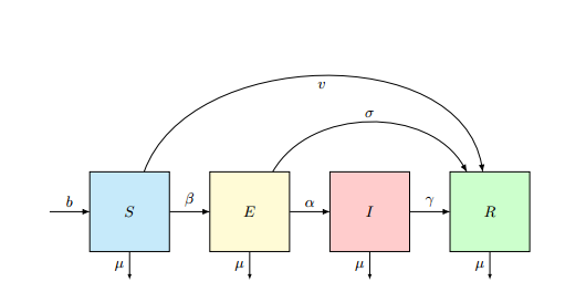
Figure 1. Flow Diagram of Measles Disease in a Deterministic Population.
Figure 1, shows flow diagram of measles disease in a deterministic population. Where the model variables and their meaning are presented in Table 1.
Table 1. State variables used and their meanings.
Variable
Meaning
\(S(t)\)
The number of susceptible individuals at a given time, t
\(E(t)\)
The number of exposed individuals at a given time, t
\(I(t)\)
The number of infective individuals at a given time, t
\(R(t)\)
The number of recovered individuals at a given time, t
Susceptible compartment includes individuals who are at risk of developing measles infection if they had contact with infected individuals. Exposed class consists of individuals that had the infection but are not showing the symptoms of the measles disease and could not transmit the disease to others. Infective compartment consists of individuals that are showing the symptoms of the disease and can infect others.
The recovered human compartment comprises of individuals who have recovered from the disease and had permanent immunity.
The susceptible class \(S\) is increasing by recruitment (birth and/or immigration rate) which we denoted by \(b\). It is decreasing by susceptible class who have been immunized by the rate \(v\), is decreasing by infection if there is a contact with infected individuals at a rate of \(\beta\), and is diminishing by leaving (normal death and emigration) rate which we denoted by \(\mu\) so that:
\begin{eqnarray}\label{succeptible_class}
\frac{dS}{dt} = b – \beta SI – ( v + \mu) S
\end{eqnarray}
(2)
For the second class, Exposed \(E\), the individuals here is formed by direct contact with infected individuals at a rate of \(\beta\). We define parameters and their meaning in Table 2 below.
Table 2. State parameters and their meaning.
Parameter
Meaning
\(b\)
Recruitment rate ( by birth and/or immigrants)
\(v\)
vaccination rate for the susceptible class who later got vaccinated
\(\mu\)
Leaving rate (by death and/or emigrants)
\(\beta\)
The contact rate
\(\gamma\)
The rate at which an infective individuals recovered per unit time
\(\sigma\)
The rate of exposed individuals who have undergone testing and therapy
\(\alpha\)
The rate at which an exposed become infective
The class \(E\) is decreasing by individuals who have undergone testing and measles therapy at a rate of \(\sigma\), the individuals who progresses into infected class at a rate of \(\alpha\) and also this class is diminishing by leaving rate of \(\mu\) so that:
The third class \(I\), of infective individuals is formed by individuals who progresses from exposed class to this class
at a rate \(\alpha\). This class is decreasing by individuals who are recovering from infection at a
rate of \(\gamma\) and is diminishing by leaving rate of \(\mu\). We then have that:
\begin{eqnarray}\label{infected}
\frac{dI}{dt} = \alpha E – (\mu + \gamma)I
\end{eqnarray}
(4)
From the SEIR model, it is assumes that Susceptible-immunized individuals, Exposed-Recovered individuals and Infected-Recovered individuals become immune to the measles disease permanently, i.e. you can only be infected once with the disease. We use this assumption to generates the fourth class \(R\) of individuals who have complete protection against the disease. This class \(R\) of recovered individuals is diminishing by leaving rate of \(\mu\). So that:
\begin{eqnarray}\label{recovered}
\frac{dR}{dt} = v S + \gamma I + \sigma E – \mu R
\end{eqnarray}
(5)
This SEIR model is now represented by the following system of first order differential equations and shows the transitions between the four compartments of the model:
\begin{equation}\label{model1}
\begin{cases}
\frac{dS}{dt} = b – \beta SI – (v + \mu) S,\\
\frac{dE}{dt} = \beta SI – (\mu + \alpha + \sigma)E\\
\frac{dI}{dt} = \alpha E – (\mu + \gamma)I\\
\frac{dR}{dt} = v S + \gamma I + \sigma E – \mu R
\end{cases}
\end{equation}
(6)
2.1. Model assumptions
The following are the assumptions for the compartmental SEIR model for measles disease which we modeled in this work:
(i) The recruitment rate (which is through newborns and/or migrants) are assumed to be susceptible to the disease.
(ii) We assumed that every person in the population under consideration is susceptible to the measles disease.
(iii) Every Individual is equally likely to be infected by the infectious individual (s) in a case of contact except for those who are immune against the measles disease.
(iv) Infectious individuals are detected early and isolated for immediate treatment and education
(v) The population is homogeneously mixed. By homogeneously mixed we mean a population that interacts among themselves in such a uniformly manner.
(vi) The population is a varying population where recruitment rate and leaving rate are differ within a given time steps.
(vii) There is no treatment failure, a patient will either recover or die.
(viii) Recovered individuals are permanently immune against the disease.
2.2. Properties of the model
The basic properties of our model are that of the properties of “feasible solution” and “positivity of the solution”. The feasible solution of the model equations shows the region in which the solution of the equations are biologically significant and the positivity of the solutions tells the non-negativity of the solutions of the model equations.
2.3. Feasible solution
Here, the deterministic SEIR model is used to model infectious disease in a human population. It will be reasonable to assumed that the parameters used and variables in all classes are non negative, that is \(t \geq 0\). The show that all variables of the model are non-negative for all given non-negative initial conditions are provided below. The feasible solution region which is positively invariant set of the model is given by:
Lemma 1.
The set \(\Omega\) is positively invariant and attracts all solution in \(\mathbb{R}_{+}^{4}\).
Proof.
Since \(N(t) = S(t) + E(t) + I(t) + R(t)\). Adding Equations (2) to (5) together gives us the rate of change of the total population:
\begin{align*}
\frac{dN}{dt} &= \frac{dS}{dt} + \frac{dE}{dt} + \frac{dI}{dt} + \frac{dR}{dt} \\
&= b – \mu(S+E+I+R)\\
&= b – \mu N \hspace{1cm} (since \hspace{0.1cm} N \hspace{0.1cm} = S+E+I+R).\end{align*}
This is a first order linear differential equation and a first order linear differential equation of the form
\begin{equation}\label{2.7}
\frac{dN}{dt}+ \mu N = b \hspace{1cm} (After \hspace{0.2cm} re-arranging)
\end{equation}
(8)
can be solved by introducing integrating factor. Here, \(\mu\) and \(b\) are both constants, so the integrating factor \(I.F\) is given as:
\(I.F= \exp \bigg(\int \mu dt \bigg).\) Now multiplying both sides of Equation (8) with \(\exp(\int \mu dt)\) given,
\begin{equation}\label{2.77}
\exp \bigg(\int \mu dt \bigg) \bigg( \frac{dN}{dt} + \mu N \bigg) = b \exp \bigg(\int \mu dt \bigg).
\end{equation}
(9)
The left hand side of Equation (9) is
\( \frac{d}{dt} \bigg[ N(t). \exp \bigg(\int\mu dt \bigg)\bigg]\),
therefore
\[ \frac{d}{dt} \bigg[ N(t). \exp \bigg (\int\mu dt \bigg) \bigg] = b . \exp \bigg( \int \mu dt \bigg) \]
Integrating both sides, we have
\[ N(t). \exp (\mu dt) = \frac{b}{\mu} \exp (\mu dt) + K,\]
where \(K\) is a constant. So that
\[N(t) = \frac{b}{\mu} + K\exp(-ut) . \]
When \(t=0\), we have that
\[ N(0) = \frac{b}{\mu} + K. \]
Therefore,
\[ K = N(0) – \frac{b}{\mu}\,. \]
Substituting the value of \(K\), the solution (with simplification) of this linear differential equation will becomes:
\[ N(t) = N(0)\exp^{-\mu t}+ \frac{b}{\mu} (1- \exp(-\mu t)). \]
Taking the limit as \(t \rightarrow \infty\), we have
\[ N(t) \leq \frac{b}{\mu}.\]
Therefore, we have established that \(\Omega\) is positively invariant and attracts all solution in \(\mathbb{R}_{+}^{4}\).
2.3.1 Positivity of results
In this section we prove that all variables in the SEIR model Equations (2) to (5) are non-negative.
Lemma 2.
Let the initial data set be \((S, E, I, R) (0) \geq 0 \in \Omega\), then the solution set \((S(t), E(t), I(t), R(t) ) \) of the equations (2) to (5) is positive \(\forall\]t > 0\).
Proof.
From Equation (2) if we assumed that:
\[\frac{dS}{dt} = b – \beta SI – (v + \mu) S \geq -(\beta SI + v + \mu S ).\]
That is
\[\frac{dS}{dt} \geq -(\beta I + v + \mu )S \hspace{0.5cm} or \hspace{0.5cm} \frac{dS}{S} \geq -(\beta I + v + \mu )dt \hspace{1cm} (by \hspace{0.1cm} separation \hspace{0.1cm} of \hspace{0.1cm} variables, \hspace{0.1cm} since \hspace{0.1cm} S \ne 0) .\]
Integrating both sides of the inequalities, we have
\[In \big( S(t) \big) \geq -(\beta I + v + \mu )t + K.\]
So that
\[S(t) \geq K \exp \bigg( -(\beta I + v + \mu )t\bigg). \]
At \(t = 0\); this becomes:
\[S(t) \geq S(0) \exp \bigg( -(\beta I + v + \mu )0\bigg) \geq 0 \hspace{1cm} (since \hspace{0.1cm} (\beta I + v + \mu ) > 0).\]
That is
\[ S(t) > 0.\]
Similarly from Equation (3), we have
\[\frac{dE}{dt} = \beta SI – (\mu + \alpha + \sigma)E \geq – (\mu + \alpha + \sigma)E \]
i.e.,
\[\frac{dE}{dt} \geq – (\mu + \alpha + \sigma)E \]
or
\[\frac{dE}{E} \geq – (\mu + \alpha + \sigma)dt \hspace{1cm} (by \hspace{0.1cm} separation \hspace{0.1cm} of \hspace{0.1cm} variables, \hspace{0.1cm} since \hspace{0.1cm} E \ne 0) .\]
Integrating both sides of the inequalities we have;
\[ E(t) \geq K \exp \bigg(- (\mu + \alpha + \sigma)t \bigg).\]
At \(t = 0\), we have that
\[E(t) \geq E(0) \exp \bigg(- (\mu + \alpha + \sigma\bigg)0 \geq 0, \hspace{1cm} (since \hspace{0.1cm} (\mu + \alpha + \sigma) > 0.\]
That is
\( E(t) > 0.\)
Also from Equation (4), we have
\[\frac{dI}{dt} = \alpha E – (\mu + \gamma)I \geq – (\mu + \gamma)I.\]
That is
\[\frac{dI}{dt} \geq – (\mu + \gamma)I.\]
Then we have that:
\[\frac{dI}{I} \geq – (\mu + \gamma)dt.\]
On integrating we obtains
\[ In \big( I(t) \big) \geq – (\mu + \gamma)t + K,\]
that is
\[I(t) \geq K \exp \bigg(- (\mu + \gamma)t \bigg).\]
At \(t=0\), we have
\(I(t) \geq I(t) \exp \bigg(- (\mu + \gamma)0 \bigg).\)
So that
\( I(t) > 0.\)
Finally from Equation (5), we have
\[\frac{dR}{dt} = v S + \gamma I + \sigma E – \mu R > \sigma E – \mu R.\]
That is,
\[\frac{dR}{dt} > \sigma E – \mu R.\]
Which has an integrating factor \( I.F = \exp (-\mu t).\) Then we have:
\[\frac{dR}{dt}.\exp (-\mu t) > \sigma E. \exp (-\mu t) – \mu R . \exp (-\mu t).\]
Integrating at constant \(K\), we have
\[ R(t) > \frac{\sigma E}{\mu} + K \exp (-\mu t).\]
When \(t=0\) we obtained that
\(R(0) >\frac{\sigma E}{\mu} + K.\)
The solution then becomes
\[R(t) > R(0)\exp (-\mu t) +\frac{\sigma E}{\mu} (1- \exp (-\mu t)).\]
That is
\(R(t) > 0.\)
Hence, we have proved that all variables are positive \(\forall t > 0\).
2.4. Existence and uniqueness of solution for the SEIR model
One will be interested in asking the following questions:
(1) Under what conditions, the solution to Equation (10) exists?
(2) Under what conditions, there is a unique solution to Equation (10)?
To answers these, let
\begin{equation*}
\begin{cases}
f_1 = b – \beta SI – \mu S,\\
f_2 = \beta SI – (\mu + \alpha + \sigma)E,\\
f_3= \alpha E – (\mu + \gamma)I,\\
f_4 = \gamma I + \sigma E – \mu R.
\end{cases}
\end{equation*}
We use the following theorem to established the existence and uniqueness of solution for our SEIR model.
Theorem 1.[Uniqueness of Solution]
Suppose \(D\) denotes the domain, and
then whenever the pairs \((t, x_1)\) and \((t, x_2 )\) belong to the domain \(D\), where \(k\) is used to represent a positive constant, there exist a constant \(\delta > 0\) such that there exists a unique (exactly one) continuous vector solution \(x(t)\) of the system (10) in the interval \(|t – t_0 | \leq \delta\).
It is important to note that condition (12) is satisfied by requirement that \( \bigg \{ \frac {\partial{f_i}}{\partial{x_j}},\hspace{0.2cm} _{ i, j = 1, 2, …, n},\)
is continuous and bounded in the domain \(D\).
Lemma 3.
If \(f (t, x)\) has continuous partial derivative \(\frac{\partial{f_i}}{\partial{x_j}}\) on a bounded closed convex domain \(\mathbb{R}\) (i.e, convex set of real numbers), where \(\mathbb{R}\) is used to denotes real numbers, then it satisfies a Lipschitz condition in \(\mathbb{R}\).
so, we look for a bounded solution of the form
\(0 < \mathcal{R} < \infty.\)
We now prove the following existence theorem.
Theorem [Existence of solution]
Let \(D\) denote the domain defined in (11) such that (12) and (13) hold. Then, there exist a solution of model system of Equations (2)-(5) which is bounded in the domain \(D\).
Proof.
Let
\begin{equation}
f_1 = b – \beta SI – (v + \mu ) S,
\end{equation}
\begin{equation}
f_3= \alpha E – (\mu + \gamma)I,
\end{equation}
(16)
\begin{equation}
f_4 = v S + \gamma I + \sigma E – \mu R
\end{equation}
(17)
We shows that
\(\frac{\partial{f_i}}{\partial{x_j}},\hspace{0.2cm} i,j=1,2,3,4\) are continuous and bounded.
We explored the following partial derivatives for all the model equations.
From Equation (14);
\[ \bigg|\frac{\partial f_1}{\partial S}\bigg| = \bigg|-\beta I – v – \mu \bigg| < \infty,
\hspace{0.3cm}
\bigg|\frac{\partial f_1}{\partial E}\bigg| = |0| < \infty,
\hspace{0.3cm} \bigg|\frac{\partial f_1}{\partial I}\bigg| = \bigg|-\beta S \bigg| < \infty,
\hspace{0.3cm}
\bigg|\frac{\partial f_1}{\partial R}\bigg| = |0| < \infty.\]
Similarly, from Equation (15):
\[ \bigg|\frac{\partial f_2}{\partial S}\bigg| = \bigg|\beta I \bigg| < \infty,
\hspace{0.3cm} \bigg|\frac{\partial f_2}{\partial E}\bigg| = \bigg|-(\mu + \alpha + \sigma) \bigg| < \infty,
\hspace{0.3cm} \bigg|\frac{\partial f_2}{\partial I}\bigg| = \bigg|\beta S \bigg| < \infty,
\hspace{0.3cm}
\bigg|\frac{\partial f_2}{\partial R}\bigg| = |0| < \infty.\]
Also from Equation (16);
\[ \bigg|\frac{\partial f_3}{\partial S}\bigg| = |0| < \infty, \hspace{0.3cm}
\bigg|\frac{\partial f_3}{\partial E}\bigg| = |\alpha| < \infty,\hspace{0.3cm}
\bigg|\frac{\partial f_3}{\partial I}\bigg| = |- (\mu + \gamma)| < \infty,\hspace{0.3cm} \bigg|\frac{\partial f_3}{\partial R}\bigg| = |0| < \infty.\]
Finally, from Equation (17):
\[ \bigg|\frac{\partial f_4}{\partial S}\bigg| = |v| < \infty,\hspace{0.3cm} \bigg|\frac{\partial f_4}{\partial E}\bigg| = |\alpha| < \infty,\hspace{0.3cm} \bigg|\frac{\partial f_4}{\partial I}\bigg| = |\gamma| < \infty,\hspace{0.3cm} \bigg|\frac{\partial f_4}{\partial R}\bigg| = |-\mu| < \infty.\]
We have clearly established that all these partial derivatives are continuous and bounded, hence, by Theorem \ref{thm1}, we can say that there exist a unique solution of (2) to (5) in the region \(D\).
2.5. Existence of steady states of the system
Under this section we will find the equilibrium points and established asymptotic stability of the SEIR model. In order to obtained the equilibrium points of the system, we equate the system of equations of the model to zeros;
i.e.;
2.6. Stability of the SEIR model (local asymptotic stability)
To find the local stability of the model, we first find the equilibrium points (disease free equilibrium) of the system (2) to (5). By equating the system to zeros we have
\begin{equation}
b – \beta SI – (v + \mu) S = 0,
\end{equation}
\begin{equation}
\alpha E – (\mu + \gamma)I = 0,
\end{equation}
(21)
\begin{equation}
v S + \gamma I + \sigma E – \mu R = 0.
\end{equation}
(22)
From Equation (19), we have \( b = \beta SI + (v + \mu) S \equiv (\beta I + v + \mu) S\)
which implies that \( S = \frac{b}{\beta I + v + \mu}\) but at the initial state, \(v =0\) and \(\beta = 0,\) which implies
\(
S = \frac{b}{\mu}.
\)
Now from Equation (20), we have \( \beta SI = (\mu + \alpha + \sigma)E,\) which implies that
\( E = \frac{\beta SI}{(\mu + \alpha + \sigma)},\)
hence
\( E = 0\) (since \(\beta = 0\)).
Similarly from Equation (21), we have \( \alpha E = (\mu + \gamma)I,\)
which implies that \( I = \frac{\alpha E}{(\mu + \gamma)},\) hence
\( I = 0\) (since \(E = 0 \)).
Finally from Equation (22), we have
\( v S + \gamma I + \sigma E = \mu R,\)
which implies that,
\( R = \frac{ v S + \gamma I + \sigma E}{\mu}, \) hence \(R = 0\) (since \(v, I\) and \(E = 0\)).
Thus we have disease free equilibrium for this SEIR model which is given by
\(\mathcal{P}_0 = \bigg(\frac{b}{\mu}, 0, 0, 0 \bigg).\)
Note 1.
We assumed \(b \ne \mu\) for this model.
2.7. The basic reproduction number \(R_0\)
The basic reproduction number \(R_0\) of an infection can be thought of as the number of cases one measles infection case can generates on average over the course of its infectious period, in an otherwise uninfected (susceptible) population\footnote{Source: Wikipedia}.
We determined the basic reproduction number \(R_0\) by employing the method of next generation matrix.
We considered only the two infected classes in our model; the Exposed \(E\) and the Infectious \(I\) compartments. That is \(m = 2\). Define \(G = F V^{-1}\), therefore \(R_0 = \rho (F V^{-1})\) where \(\rho (F V^{-1})\) is called the spectral radius of \(FV^{-1}\). ({The spectral radius is the maximum of the absolute value of the eigenvalues}.)
Let
\(H'(x) = \mathcal{F}(x) – \mathcal{V}(x),\)
which gives
\begin{eqnarray}
\mathcal{F}(x) = \begin{bmatrix}
\beta SI \\
0 \\
\end{bmatrix}
\hspace{0.2cm}\text{and} \hspace{0.2cm}
\mathcal{V}(x) = \begin{bmatrix}
(\mu + \alpha + \sigma) E \\
\alpha E – (\mu +\gamma) I \\
\end{bmatrix}\,.
\end{eqnarray}
(23)
Taking the Jacobian of \(\mathcal{F}(x)\) and \(\mathcal{V}(x)\) respectively at the disease free equilibrium \(\mathcal{P}_{0}\), we obtained
We can easily obtain the value of \(R_0\) using the values provided in Table 3. If \(R_0 1\), the measles disease is endemic.
Let’s define
\[ R_0 = \frac{b \beta \alpha}{\mu (\mu + \alpha +\sigma)(\mu + \gamma)} \hspace{0.3cm} \text{where:} \hspace{0.2cm}
\mu (\mu + \alpha +\sigma)(\mu + \gamma) \ne 0\,.\]
2.8. Interpretation of \(R_0\)
\(R_0\) is used to explained the fact that the transmission rate, that is, the rate at which exposed individuals will become infected and the contact rate, i.e.; the average number of effective contacts with other (susceptible) individuals per infective individuals per unit time which is relative to the rate at which an infectious individuals will recovered per unit time plays a significant role in determining whether or not the measles epidemic will occur in a given human population. Thus, the disease free equilibrium \((\frac{b}{\mu}, 0, 0, 0)\) is locally asymptotically stable given that \(Ro < 1\), that is, \(b \beta \alpha 1\), then the disease free equilibrium is unstable, i.e., the system is said to be uniformly persistent, in other words the measles disease is endemic. Hence, \(R_0\) is a threshold parameter for the model that will determines the number of equilibria.
2.9. Endemic Equilibrium
The next thing in our analysis is to shows that an endemic equilibrium:
and we also show that if \(Ro > 1\), the measles disease is endemic.
From our equilibrium Equations (19) to (22), considering Equations (20) and (21), we have that:
\[\beta SI = (\mu + \alpha + \sigma)E,\;\;\;\;(\mu + \gamma)I = \alpha E.\]
Which when we divide the first by the second yields,
\[S = S^* = \frac{(\mu + \alpha + \sigma) (\mu + \gamma)}{\alpha}.\]
That is,
\[S^* = \frac{(\mu + \alpha + \sigma) (\mu + \gamma)}{\alpha},\]
which is clearly greater than zero.
Similarly, adding Equations (19) and (20), we have
\[ (v + \mu) S = b – E (\mu + \alpha + \sigma)\]
which implies
\begin{equation*}
S = \frac{ – (\mu + \alpha + \sigma)E + b}{ (v + \mu)}.
\end{equation*}
But for \(v = 0 \), we have
We have shown that \(S^*\), \(E^*\), \(I^*\) and \(R^*\) are all positives meaning that \(P^* = (S^* , E^* , I^* ,R^* ) > 0. P^*\) represent an endemic steady state with constant number of people in the population being infected with the measles disease and if \(Ro > 1\), the measles disease is endemic.
This will be biologically reasonable when \(S^* 1.\)
In another words, the necessary and sufficient condition for a unique \(P^*\) to exist in the feasible region \(\Omega\) is that
\( 0 < S^* \leq \frac{b}{\mu}.\)
or equivalently
\(\frac{b}{\mu} \geq 1.\)
2.10. Local asymptotic stability
We established the local stability of the disease-free equilibrium using Jacobian matrix of Equations (2) to (5) and evaluate at disease free equilibrium \(\mathcal{P}_0\). We achieve this by evaluating the Jacobian matrix of Equations (2) to (5) at \(\mathcal{P}_0 = (\frac{b}{\mu}, 0, 0, 0)\). The local stability of the model is determined from the eigenvalues of the Jacobian matrix of the model equations at \(\mathcal{P}_0\).
Thus, the Jacobian matrix of Equations (2) to (5) is given by
The disease free equilibrium, \(\mathcal{P}_0\), is locally asymptotically stable if all the eigenvalues of \(J(\mathcal{P}_0)\) are \( < 0\). We will establish this by finding the eigenvalues. To find the eigenvalues, take \(|J(\mathcal{P}_0) – \lambda I_4 | = 0\), then
\begin{center}
Simplify (37) gives \(\lambda_1 = -\mu,\hspace{.2cm} \lambda_2 = -\mu,\hspace{.2cm} \lambda_3 = -(\mu + \sigma + \alpha) ,
\lambda_4 = -\bigg( \frac{b \beta \alpha}{\mu} + \mu + \gamma \bigg).\)
Since the eigenvalues for \(J(\mathcal{P}_0)\) are negative so the disease free equilibrium is locally asymptotically stable.
2.11. Application of \(R_0\) to measles in Nigeria.
A deterministic compartmental mathematical model for measles has been formulated with the aim of the study of the effects of heterogeneous mixing, transmission and control (or elimination) of the disease in Nigeria. Moreover, the basic reproduction number, \(R_0\), has been derived, which is the threshold parameter.
Recall that
We will substitute the values of \(\alpha\), \(\beta\), \(b\), \(\mu\), \(\alpha\), \(\sigma\) and \(\gamma\) into \(R_0\) to investigate the behaviour of \(R_0\) with the given parameters in Table 3 which are pertinent to measles in Nigeria.
It is easy to check that when \(\sigma = 0\) we have
\( R_0 = 1.8105;\) when \(\sigma = 0.25\)
we have \( R_0 = 0.69364\); when \(\sigma = 0.50\),
We have \( R_0 = 0.42900\) and finally, when \(\sigma = 0.75\)
we have \( R_0 = 0.31053 .\)
In summary, when \(\sigma = 0\) we have \(R_0 > 1\) and when \(\sigma \le 1\) we have \(R_0 < 1\). This illustrate the fact that \(\sigma\), which is the rate of exposed individuals who have undergone testing and therapy, will play a significant role in controlling (and eliminating) of the disease.
Thus, the disease free equilibrium \((\frac{b}{\mu}, 0, 0, 0)\) is locally asymptotically stable when \(Ro < 1\) for \(\sigma \le 1\) , that is, \(b \beta \alpha 1\), then the disease-free equilibrium is unstable, i.e., the measles disease will be endemic in the population.
Hence, we have established the fact that \(R_0\) is a threshold parameter for the model that will determine the number of equilibria.
3. Numerical results
In this section, we consider the explicit fourth-order Runge-Kutta (RK4) scheme for solving numerically the non-linear first order ordinary differential equations (ODEs) of our SEIR model of Equations (6) with given initial conditions. Here, numerical simulations are used to show the impact of vaccination and therapy using the RK4 scheme on the state equations. Details of the RK4 are discussed in [15]. State equations are solved over a simulated period of time using the RK4 scheme. The parameters used in the simulation are in the Table 3.
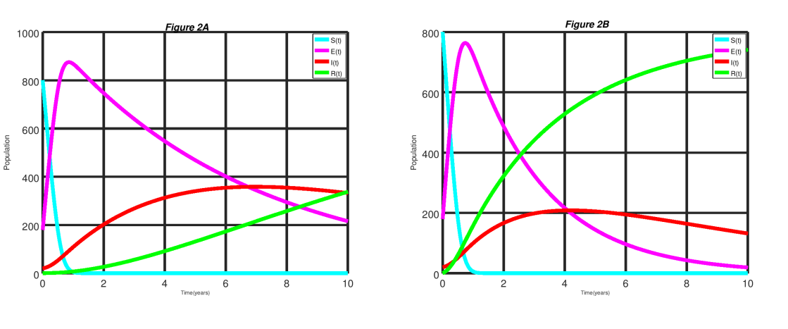
The simulation results are depicted in Figures 2 to 5.
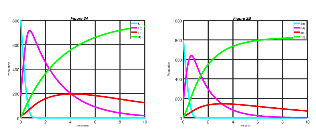
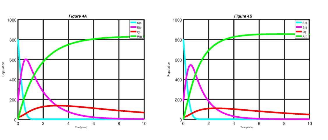
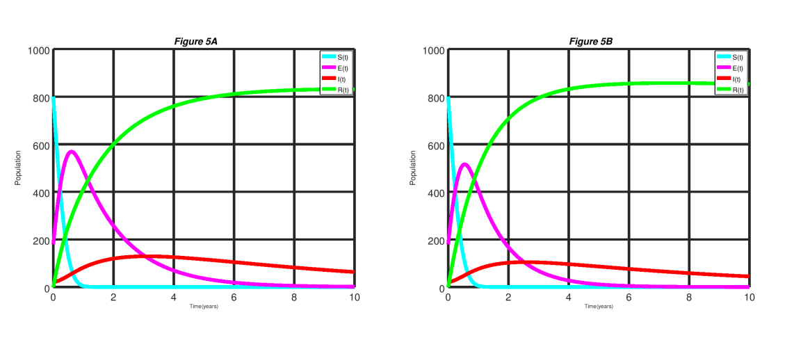
Figure 2. Measles dynamics is shown when \(\sigma\) = 0.0 and v = 0.0 (left) and when \(\sigma\) = 0.25 and v = 0.0 (right)Figure 3. Measles dynamics is shown when \(\sigma\) = 0.25 and v = 25 (left) and when \(\sigma\) = 0.50 and v = 0.25 (right)Figure 4. Measles dynamics is shown when \(\sigma\) = 0.50 and v = 0.50 (left) and when \(\sigma\) = 0.75 and v = 0.50 (right)Figure 5. Measles dynamics is shown when \(\sigma\) = 0.50 and v = 0.75 (left) and when \(\sigma\) = 0.75 and v = 0.75 (right)
3. 1. Interpretation of Simulation Results
In Figure 2 we present the dynamics of measles disease when \(\sigma = 0.0\) and \(v = 0 \) and when \(\sigma = 0.25\) and \(v = 0\). We can see in the Figure 2 that, if none of the exposed individuals at the latent period are diagnosed and treated, and there is no control measure been introduced into the susceptible class. It will take a much longer time for exposed individuals to decrease.
Likewise, it takes a significantly longer period before we notice any significant improvement for individuals to recovered from the measles disease. Similarly, infective individuals will significantly increase before noticing a drop in the number of infective individuals. On the order hand, when \(25\%\) of the exposed individuals at the latent period are diagnosed and treated, there is a clear improvement in the result.
In Figure 3, we do the simulation of the model when \(\sigma = 0.25\) and \(v = 25\) and when \(\sigma = 0.50\) and \(v = 0.25\). It can be observed from Figure 3 that if \(25\%\) of susceptible individuals are vaccinated in addition to increases of \(25\%\) to \(50\%\) of the exposed individuals at the latent period who are diagnosed and treated. It will take lesser time for exposed individuals to decrease significantly. Also, it takes a significant lesser period before noticing any significant improvement for individuals to recovered from the disease. Similarly, infective individuals will significantly decline over time.
Figure 4, above shows the dynamics of measles disease when \(\sigma = 0.50\) and \(v = 50\) and when \(\sigma = 0.75\) and \(v = 0.50\). From the simulation result of the Figure 4, if \(50\%\) of susceptible individuals are vaccinated in addition to increases of \(50\%\) to \(75\%\) of the exposed individuals at the latent period, who are diagnosed and treated,. There is a sudden decline of exposed individuals with time. This shows a significantly improved result in comparison with what we have in the two figures above. Also, it takes a significant much lesser period for individuals to recover from the disease. Similarly, infective individuals will significantly take a lesser period to go down over time.
Figure 5 shows the simulation of the model when \(\sigma = 0.50\) and \(v = 75\) and when \(\sigma = 0.75\) and \(v = 0.75\). Looking at the Figure 5 closely, we discovered that if \(75\%\) of exposed individuals at the latent period are diagnosed and treated. In addition to increases of \(50\%\) to \(75\%\) of susceptible individuals who are vaccinated, we have a better result in comparison to the previous three results stated above.
Conclusion
The SEIR model showed significant success in attempting to predict the causes of measles disease transmission within a given population. The model strongly indicated that the spread of disease largely depends on the contact rates of susceptible individuals with infected individuals within a population. With the assumed values for our state variables, we modelled a measles disease in Nigeria using deterministic SEIR model to investigate the impact the control measures can have on susceptibles, as well as exposed individuals at latent period, over the entire population dynamics in controlling and eliminating the disease. Consequently, we established the existence of a solution, uniqueness of the solution, and stability of the solution. The application of \(R_0\) to measles data of Nigeria was also given. Finally, numerical simulations of the model with the RK4 scheme was well presented.
Acknowledgments
We appreciate the support given to us by African Institute for Mathematical Sciences (AIMS), Senegal. All the authors are well appreciated for their contributions.
Author Contributions
All authors contributed equally to the writing of this paper. All authors read and approved the
final manuscript.
Competing Interests
The author(s) do not have any competing interests in the manuscript.
References
Measles transmission mode. (October 2018). Retrieved from https://www.cdc.gov/measles/about/transmission. html.
Measles disease and transmission mode. (September 2018). Retrieved from https://www.ncdc.gov.ng/diseases /info/M.
Immunization Misconceptions. (September 2019). Retrieved from https://www.who.int/vaccine\_safety/initiative/
detection/immunization\_misconceptions/en/
Measles Outbreak in Nigeria. (2019). Retrieved from
https://reliefweb.int/report/nigeria/nigeria-measles-outbreak- dg-echo-who-ncdc-ngos-echo-daily-flash-16-march-2019.
Hethcote, H. W. (2000). The mathematics of infectious diseases. SIAM review, 42(4), 599-653.[Google Scholor]
Bakare, E. A., Adekunle, Y. A., & Kadiri, K. O. (2012). Modelling and Simulation of the Dynamics of the Transmission of Measles. International Jounal of Computer Trends and Technology, 3, 174-178.[Google Scholor]
Bolarian, G. (2014). On the dynamical analysis of a new model for measles infection. International Journal of Mathematics Trends and Technology, 7(2), 144-155.[Google Scholor]
Fred, M. O., Sigey, J. K., Okello, J. A., Okwoyo, J. M., & Kang’ethe, G. J. (2014). Mathematical modeling on the control of measles by vaccination: Case Study of KISII County, Kenya. The SIJ Transactions on Computer Science Engineering and Its Applications (CSEA), 2, 61-69.[Google Scholor]
Roberts, M. G., & Tobias, M. I. (2000). Predicting and preventing measles epidemics in New Zealand: application of a mathematical model. Epidemiology & Infection, 124(2), 279-287.[Google Scholor]
Momoh, A. A., Ibrahim, M. O., Uwanta, I. J., & Manga, S. B. (2013). Mathematical model for control of measles epidemiology. International Journal of Pure and Applied Mathematics, 87(5), 707-717.[Google Scholor]
Tessa, O. M. (2006). Mathematical model for control of measles by vaccination. In Proceedings of Mali Symposium on Applied Sciences (Vol. 2006, pp. 31-36).[Google Scholor]
Momoh, A. A., Ibrahim, M. O., Uwanta, I. J., & Manga, S. B. (2013). Mathematical model for control of measles epidemiology. International Journal of Pure and Applied Mathematics, 87(5), 707-717.[Google Scholor]
Ochoche, J. M., & Gweryina, R. I. (2014). A mathematical model of measles with vaccination and two phases of infectiousness. IOSR Journal of Mathematics, 10(1), 95-105.[Google Scholor]
Verguet, S., Johri, M., Morris, S. K., Gauvreau, C. L., Jha, P., & Jit, M. (2015). Controlling measles using supplemental immunization activities: a mathematical model to inform optimal policy. Vaccine, 33(10), 1291-1296.[Google Scholor]
Sowole, S. O., Sangare, D., Ibrahim, A. A., & Paul, I. A. (2019). On the existence, uniqueness, stability of solution and numerical simulations of a mathematical model for measles disease, International Journal of Advances in Mathematics, 2019(4), 84-111.[Google Scholor]
Nigeria-population: Worldometers on world population. (October 2019). https://www.worldometers.info/world- population/nigeria-population/
Nigeria birth rate from index mundi. (September 2019). Retrieved from https://www.indexmundi.com/ nigeria/birth\_rate.html
Nigeria Migration Profile. (September 2019). Retrieved from https://www.dailytrust.com.ng/more-foreign-visitors- troop-into-nigeria-data.html.[Google Scholor]
Nigeria death rate from index mundi. (September 2019) . Retrieved from https://www.indexmundi.com/nigeria /death\_rate.html.
Trottier, H., & Philippe, P. (2003). Deterministic modeling of infectious diseases: measles cycles and the role of births and vaccination. The Internet Journal of Infectious Diseases, 1(2), https://print.ispub.com/api/0/ispub-article/7099.[Google Scholor]