This paper studies the movement of a molecule in two types of cell complexes: the square tiling and the hexagonal one. This movement from a cell \(i\) to a cell \(j\) is referred to as an homogeneous Markov chain. States with the same stochastic behavior are grouped together using symmetries of states deduced from groups acting on the cellular complexes. This technique of lumpability is effective in forming new chains from the old ones without losing the primitive properties and simplifying tedious calculations. Numerical simulations are performed using R software to determine the impact of the shape of the tiling and other parameters on the achievement of the equilibrium. We start from small square tiling to small hexagonal tiling before comparing the results obtained for each of them. In this paper, only continuous Markov chains are considered. In each tiling, the molecule is supposed to leave the central cell and move into the surrounding cells.
Living organisms consist of one or more tiny components of several types and shapes termed
cells on which molecules move in continuous random motion. These cells and the molecules can
be considered as subdivisions of a 2-dimensional plane on which particles randomly move. The
plane can be much wider, but considering that each molecule moving on the plane has a starting
cell, we can restrict this movement to a few groups of cells. The knowledge obtained from this small
group of cells can be extended to improve our understanding of the molecules movement on
a larger scale. The shape of the cells dictates the different random possibilities of a molecule
movement to neighboring cells from the starting cell.
A cell can assume different shapes, including square and hexagonal shapes. In both square
and hexagonal tilings assumed by a cell, the set of all possibilities of a molecule moving towards
a neighboring cell can be seen as a Markov chain \(\{X_t , t > 0\}\) [1]. This Markov chain is driven by a parameter \(p\) which represents the probability for the molecule under study to move from one cell to a neighboring cell. A Markov chain can be discrete or continuous depending on whether the time considered is discrete or continuous [2].
A recent study made in [1] on this topic considered discrete time process. It was demonstrated that the molecule is faster in the hexagonal tiling than in the square tiling.
In this paper, we will look at the continuous process and compare the result with those found in the discrete process. We will examine how the probability impacts the movement of a molecule from cell \(i\) to cell \(j\). When a molecule moves from a cell \(i\) to \(j\), the possible next step of the movement depends on the number of cells enclosing it. For example, from the central cell of the square tiling , a molecule has four possibilities to move to while there are six possibilities in the hexagonal tiling.
In the aforementioned study ([1]), two starting positions were considered: the central cell and the surrounding ones.
We only consider the central cell to be the starting position of the molecule since each cell (even the border cells) can be considered as central by enlarging the plane.
Infinitesimal generators in continuous time will replace the transition matrices in discrete time
to describe the movement of the molecule. In this study, the space is discrete.
Sometimes, the transition matrices can be very large and almost impossible to handle for doing computations. In order to reduce the calculations, we will use the state symmetries after identifying the non-equivalent cells in each tiling, then we will lump states with ²the same properties [3]. Symmetric groups afford a precise definition of structural equivalence for Markov chains states in aggregating them to making a partition
of the original Markov process in small subsets that conserve all the previous properties [4]. This aggregation results in a new Markov chain (aggregated chain) with fewer number of states such that the finite probabilities of aggregated states equals the finite
probabilities of the corresponding states of the initial Markov chain [5].
The specific questions we want to address include:
(1) What is the effect of the discrete or continuous nature of time in the oscillatory movement
of the molecule?
(2) What is the effect of the probability, the time and the shape of the tiling in the attainment of the equilibrium in continuous Markov process under consideration ?
2. Markov chains
2.1. Definitions
Definition 1.
A sequence of random variables \(\{X_n\}_{n_{\geq 0}}\) in a countable space E is called stochastic process. E is called states space whose elements will be written \textit{i, j, k, …}.
When \(X_n = i\), the process is in the state \(i\) or visits the state \(i\) at the time \(n\).
Sequences of random variables which are independent and identically distributed are stochastic process but they do not take into account the dynamic of evolution of systems due to their independence.
To introduce this dynamic, one must take into account the influence of the past, which Markov chains do, like the equation of recurrence in deterministic systems [2].
Then we introduce the following:
Definition 2.
For all \(n\in \mathbb{N}\) and all states \(i_0 , i_1, i_2, i_3,…,i_{n-1},i,j \in E\),
then the process \(\{X_n\}_{n_{\geq 0}}\) is called Markov chain.
The Equation (1) is called Markov property.
The matrix \(P=\{p_{ij}\}_{i,j\in E},\) where
\begin{equation*}
p_{ij}=P(X_{n+1}=j\arrowvert X_n =i)
\end{equation*}
is the probability to move from \(i\) to \(j\), is called transition matrix of the chain.
Since all \(p_{ij}\) are probabilities and the transition happens from a state \(i\) to a state \(j\), one has \(p_{ij}\geq 0\) and \[\sum_{k\in E} p_{ik}=1,~~ \forall i,j.\]
A matrix indexed by E and satisfying the above properties is a stochastic matrix.
A Markov chain is said to be \textit{discrete time} if the state space of the possible outcomes of the process is finite.
2.2. Continuous-time Markov chains
Definition 3.
A continuous-time Markov chain \(X(t)\) is defined by two components: a jump chain, and a set of holding time parameters \(\lambda_i.\) The jump chain consists of a countable set of states \(S\subset\{0,1,1,…\}\) along with transition probabilities \(p_{ij}\). We assume \(p_{ii}=0\), for all non-absorbing states \(i\in S\).
We assume that:
1) If \(X(t)=i\), the time until the state changes has exponential \((\lambda_i)\) distribution;
2) If \(X(t)=j\), the next state will be in \(j\) with probability \(p_{ij}\).
The process satisfies the Markov property 1.
For a continuous Markov chain, the Equation (1) can be rewritten as follows:
This chain is homogeneous if the second member of (2) does not depend on the time \(t\). If (2) is a system of differential equations that does not depend on \(t\), it is said to be an autonomous system ([6]) whose stability depends on the signs of its eigenvalues.
We can then define the transition matrix, \(P(t)\).
Assuming the states are \(1, 2,…, r\), then the state transition matrix for any \(t\geq 0\) is given by
Let \(X(t)\) be a continuous-time Markov chain with transition matrix \(P(t)\) and state space \(S=\{0,1,2,…\}\). A probability distribution \(\pi\) on \(S\) i.e, a vector \(\pi =[\pi_1, \pi_2,\pi_3,..]\), where \(\pi \in [0,1]\) and
$$\sum_{i} \pi_i = 1$$
is said to be a stationary distribution for \(X(t)\) if
The intuition here is exactly the same as in the case of discrete-time chains. If the probability distribution of \(X(0)\) is \(\pi\), then the distribution of \(X(t)\) is also given by \(\pi\), for any \(t\geq 0\).
The Equation (3) is solution to the so called backward Chapman-Kolmogorov equation below [7]
\begin{equation}\label{equation diff of probability matrix}
P'(t)=GP(t).
\end{equation}
(5)
Calculation of Equation (5) may be cumbersome and tedious. This hindrance can be overcome by using lumpability if the transition matrix satisfies some conditions (see
[8], [9] and [3]).
The following definition from [9] is important for the suit of this paper.
Definition 4.
Let \(\{X_t\}\) be a Markov chain with state space \(S=\{1,2,\cdots,r\}\) and initial vector \(\pi\). Given a partition \(\bar{S}=\{E_1, E_2, \cdots, E_v\}\) of the space \(S\), a new chain \(\bar{X}_n\) can be defined as follows: At the \(jth\) step, the state of a new chain is the set \(E_k\) when \(E_k\) contains the state of the \(jth\) step of the original chain.
Precisely, a continuous Markov chain is said to be lumpable with respect to the partition \(\bar{S}\) if for \(i,j \in E_\eta\),
According to [8], a Markov chain X whose transition probability matrix from state \(i\) to state \(j\) denoted by \(p_{ij}\) is lumpable with respect to the partition \(\bar{S}\) if and only if for every pair of sets \(E_\eta\) and \(E_\theta\), \(\sum_{k} \in E_\eta p_{ik}\) has the same value for every \(e_i\) in \(E_\theta\). These common values form the transition probabilities \(p_{\eta, \theta}\) for the lumped chain.
Moreover, one has the following theorem from [9].
Theorem 1.
Let X(t) be an irreducible continuous-time Markov chain with stationary distribution \(\pi\). If it is lumpable with respect to a partition of the state space, then the lumped chain also has a stationary distribution \(\bar{\pi}\) whose components can be obtained from \(\pi\) by adding corresponding components in the same cell of partition.
Infinitesimal Generator of Continuous-time Markov chains
The infinitesimal generator matrix, usually shown by G, gives us an alternative way of analyzing continuous-time Markov chains. Consider a continuous-time Markov chain \(X(t)\). Assume \(X(0)=i\). The chain will jump to the next state at time \(T_1\), where \(T_1\sim Exponential(\lambda_i)\). In particular, for a very small \(\delta \geq 0\), we can write
\begin{equation*}
P(T_1 \leq \delta)=1-e^{-\lambda_i \delta}\simeq 1-(1-e^{-\lambda_i \delta})
=\lambda_i\delta.
\end{equation*}
Thus, in a short interval of length, \(\delta\) the probability of leaving state \(i\) is approximately \(\lambda_i \delta\). For this reason, \(\lambda_i\) is often called the transition rate out of state \(i\). Formally, we can write
An infinitesimal generator always satisfies the equation
\begin{equation}
\sum_j g_{ij}=0.
\end{equation}
(9)
For an infinitesimal generator to be lumpable, it must satisfy the condition contained in the following definition that the reader can check in [9].
Definition 6.
We say that an infinitesimal generator G is lumpable if
\begin{equation}
\sum_{k\in E_\theta} g_{ik}=\sum_{k\in E_\theta}g_{jk},~~ for ~~i,j \in E_\eta.
\end{equation}
(10)
First hitting times
Definition 7.
Let (\(X_t)_{t\ge 0}\) be a Markov chain with generator matrix G. The hitting time
of a subset A\(\subset \)S is the random variable
$$\tau^A (\omega )=inf\{t\ge 0|X_t(\omega)\in A\}$$ with the usual convention \(inf\emptyset =\infty\).
Theorem 2.
The vector of mean hitting times \(k^A=\{ k_i^A|i\in S\}\) is the minimal nonnegative solution of
3. Investigation of the movement on small tiling in continuous time
In this section we investigate the motion of a molecule in two small tilings: the square tiling
and the hexagonal one. This movement from a cell \(i\) to a cell \(j\) is considered as being an homogeneous
Markov chain. States with the same stochastic behavior are lumped together using symmetries
of states deduced from groups acting on the cellular complexes. According to [12], the group acting on a polygon is a dihedral group. In the particular case of the small square tiling, we have the symmetric group \(S_9\) and for the hexagonal tiling we have \(S_7\). Thanks to these groups, we will use the technique of lumpability. This lumpability is effective in forming new chains from the old ones without losing the primitive properties and
simplifying tedious calculations.
At each step, the molecule is supposed to leave the central cell and move into the surrounding
cells. In [1], it is shown that the movement of biological molecule on tilings (either square or hexagonal) can be modeled by a (discrete time) Markov chain. We will extend this movement of biological molecule on small tiling in continuous time.
3.1. Continuous-time process in small square tilng
We already have important results from previous works on discrete-time Markov process in small cell complexes ([1]). We want to extend this study to the continuous case especially in the square tiling. We will assume a discrete space throughout this study.
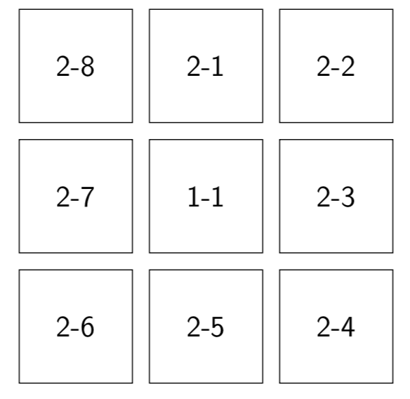
Figure 1. Small square tiling.
As already highlighted, a molecule is supposed to be at the central cell (cell 1-1 on Figure 1) at the beginning of the motion. When coming from this position, the molecule can immediately move to one of the following neighboring cells: 2-1, 2-3, 2-5 and 2-7. Thus, the probability of moving to each one of them is the same. However,to move to the cells at the corners, the molecule will move in two steps: the first is the transit to the surrounding cell and the second to the corner. This means that there is also the same probability to move to each corner cell. But this probability differs from the preceding. In the paragraph below, we analyze this to show how to reduce calculations of the infinitesimal generator.
3.1.1. Infinitesimal generator and probability matrix
The molecule has four possibilities of moving to neighboring state with, assume, probability \(p\). All cells can be reached in one step from the center except those located at the corner (corner cells) of the tiling. Therefore, the infinitesimal generator, \(G\) for a square tiling takes the form
where all \(\alpha \geq 0\) is the transition rate. This matrix corresponds to an irreducible chain because it is always possible to go from one state to another (see [13] for further details).
We now compute the probability matrix \(P(t)\) defined by Equation (3) by using the Chapman-Kolmogorov backward equation (see Equation (5)).
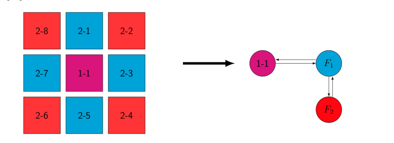
A direct computation of Equation (5) will be tedious because of the size of Equation (12). We therefore lump the symmetric states as depicted on Figure 2. This figure shows that the symmetric group \(S_9\) is a partition of the proposed Markov chain.
Figure 2. Lumpability of small square tiling
The original Markov chain is lumped as \textcolor{magenta}{(1-1)}\textcolor{cyan}{(2-1 2-3 2-5 2-7)}\textcolor{red}{(2-2 2-4 2-6 2-8)}.
The new infinitesimal generator is obtained from
The original Markov chain and the new infinitesimal generator satisfy all the hypotheses of the Definitions 4 and 6.
Substituting each parameter by its value in the Equation (13), we get the new infinitesimal generator,
Substituting Equation (14) into Equation (5), we get for
\begin{equation*}
P(t)=
\begin{pmatrix}
p_{11}& p_{12} & p_{13} \\
p_{21}& p_{22} & p_{23} \\
p_{31}& p_{32} & p_{33}
\end{pmatrix},
\end{equation*}
where all \(p_{ij}\) (\(i,j\in\{1,2,3\}\)) are functions depending on the same variable \(t\)); the following system:
This system is made of equivalent equations. Thus, instead of solving the whole system, we just solve one of the systems with three equations. We can either solve
Algebraic computations show that the matrix associated to any of the subsystems (i.e. Equation (17), Equation (18), and Equation (19) ) has three eigenvalues : \(\lambda_1 =-6\alpha,~~ \lambda_2 = -3\alpha\) and \(\lambda_3 =0\) and the corresponding eigenvectors:
$$v_1 =\begin{pmatrix}
1\\
\frac{-1}{2}\\
\frac{1}{4}
\end{pmatrix},~~~ v_2 =\begin{pmatrix}
1\\
\frac{1}{4}\\
\frac{-1}{2}
\end{pmatrix}, ~~~ v_3 =\begin{pmatrix}
1\\
1\\
1
\end{pmatrix}.$$
The general solution of each subsystem can be written as
%Equation \ref{Solution matrix expsmallsquare} can be found by computing directly the exponential of the product of \(t\) and the infinitesimal generator \(G\).
3.1.2 Stationary distribution and limiting probability
A stationary distribution of a Markov chain is a probability distribution that remains unchanged in the Markov chain as time progresses. Typically, it is represented as a row vector \(\pi\) whose entries are probabilities summing to \(1\) and, given the transition matrix \(P\), it satisfies the Equation (4).
It can be shown (see [14])that the Equation (4) is equivalent to
\begin{equation}
\label{StationaryDistribution with Inf Generator}
\pi G = 0
\end{equation}
(25)
with \(G\) the infinitesimal generator of the chain. Considering \(\pi\), the stationary distribution associated to the lumped chain above reduces the relation Equation (25) as
Solving this system (Equation (27)), we find the stationary distribution \(\pi =\left(\frac{1}{9},\frac{4}{9},\frac{4}{9}\right).\)
This stationary distribution found is exactly the same as the one associated with the original chain, i.e. non-lumped system.
Another parameter relating to stationary distribution is the limiting distribution.
Definition 8.
The limiting distribution of a Markov chain seeks to describe how the process behaves a long time after.
For the limiting distribution to exist, the following limit must exist for any states \(i\) and \(j\)
This ensures that the numbers obtained do, in fact, constitute a probability distribution. Provided these two conditions are met, then the limiting distribution of a Markov chain with \(X_0 =i\) is the probability distribution given by \(l=(L_{ij})_{states~j}\).
For any time-homogeneous Markov chain that is aperiodic and irreducible, \(\lim_{n\longrightarrow\infty} \mathbf{P}^n\)
converges to a matrix with all rows identical and equal to \(\pi\).
For time-homogeneous Markov chains, any limiting distribution is a stationary distribution [15]. The relation Equation (28) applied on the matrix
Equation (24) provides the following matrix:
$$
\mathbf{P}_{\pi}=\begin{pmatrix}
\frac{1}{9}&\frac{4}{9} & \frac{4}{9} \\
\frac{1}{9}&\frac{4}{9} & \frac{4}{9} \\
\frac{1}{9}& \frac{4}{9} & \frac{4}{9}
\end{pmatrix},
$$
which is the limiting distribution of the Markov chain deduced from the square tiling.
It is a stochastic matrix. It satisfies the Equation (29) as expected.
3.1.3. Calculation of the mean hitting times
In this section, we want to compute the mean value of the time to be spent by the molecule in a cell for the first time by using the Equation (11).
For \(A=\{1\}\), we have the following system:
\begin{equation*}
\left\lbrace \begin{array}{rrr}
k_1^A &=&0,\\
g_{21}k_1^A +g_{22}k_2^A +g_{23}k_3^A &= &-1,\\
g_{31}k_1^A +g_{32}k_2^A +g_{33}k_3^A &=&-1,\\
\end{array}
\right.
\end{equation*}
whose solution is \( \begin{pmatrix}
0 \\
\\
\frac{2}{\alpha} \\
\\
\frac{5}{2\alpha}
\end{pmatrix} \) after substituting all the \(g_{ij}\) with their corresponding values in Equation (14). In the same way, we respectively have for \(A=\{2\}\) and \(A=\{3\}\) the following vectors:
\( \begin{pmatrix}
\frac{1}{4\alpha} \\
\\
0 \\
\\
\frac{1}{2\alpha}
\end{pmatrix} \) and \( \begin{pmatrix}
\frac{7}{8\alpha} \\
\\
\frac{5}{8\alpha} \\
\\
0
\end{pmatrix}. \)
The undermentioned matrix H summarizes the findings for the mean hitting times:
3.1.5. R simulation of effect of probability and time on the movement in square tiling
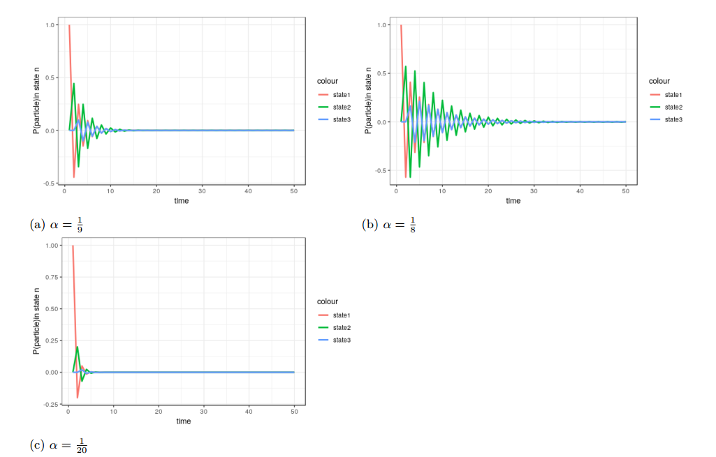
Figure 3 and 4 represent the transition rate against time. The Figure 3, in particular, shows how the variation in the transition rates affects the attainment of the equilibrium. By comparing graph 3a and graph 3c, we can see that the variation in the \(\alpha\) parameter value affects the oscillation of the state curves. This means that the variation of the transition rates influences the attainment of the equilibrium. We can notice that on the graph 3c where the probability value is the smallest, the equilibrium state is reached quicker than on the other two graphs of the same figure.
Figure 3. Visualization of the effect of the variation of the transition rates for a fixed time (time=50) in a small square tiling
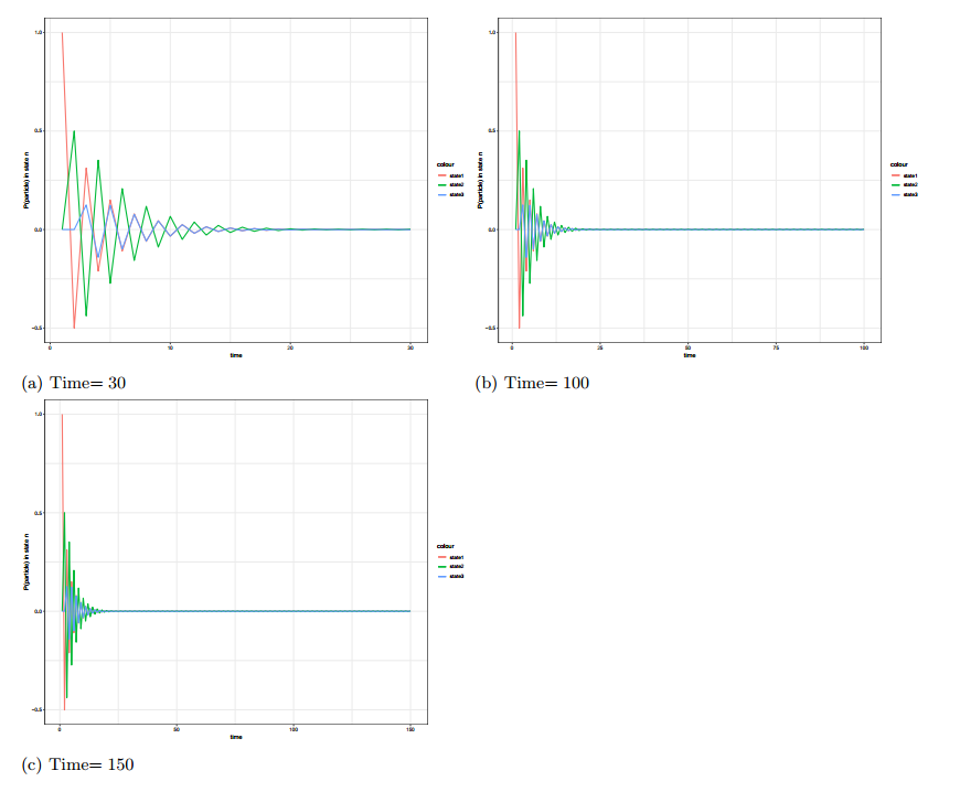
On the other hand, Figure 4, also represents the curve behavior in time variation for a fixed value of the transition rates. Hence, by comparing Figure 4a and Figure 4c we find that the slope of the state curves reaches stability at almost the fifteenth unit of time. This explains why, considering a larger time interval, the equilibrium status seems to be reached very early.
For example, if we choose the second as unit of time, we can note that from graph Figure 4a starts the equilibrium phase almost at the eighth second. Considering a larger interval of time (as 100 at Figure 4b or Figure 4c), the equilibrium attainment time is still the fifteenth second. It can be seen that the starting state curve is less steep on Figure 4a where the time is 30 than in graph 4c where the time is 150.
Figure 4. Visualization of the effect of the variation of time for a fixed transition rate (\(\alpha=\frac{1}{8}\)) in a square tiling
From these two panels of graphs, we see that the fastness in the attainment of the equilibrium is not dictated by the duration of the movement but by the value of the probability (transition rates).
4. Continuous-time process in small hexagonal tiling
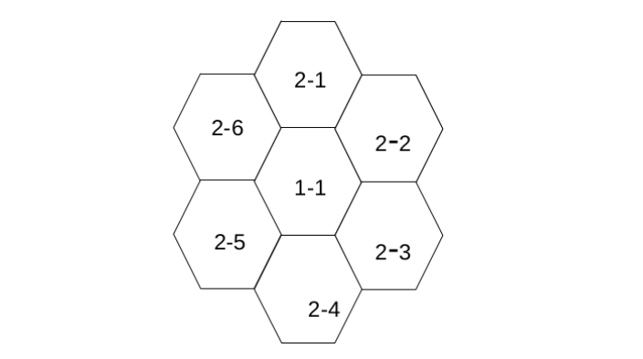
In this section, we examine how some parameters influence the behavior of the motion in the hexagonal tiling. We will consider the aggregated complex cell for reducing the computations. The unique starting position is the central cell 1-1.
4.1. Infinitesimal generator and probability matrix
Let us consider the small hexagon depicted on Equation (5). From the central cell, the molecule (the system) has six possible equiprobable destinations which are its neighboring cells. Based on this information, we then produce the following infinitesimal generator
Figure 5. Small hexagonal tiling
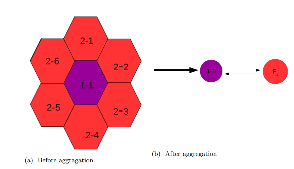
On Figure 5 we have two kinds of equivalent cells: The central cell and the surrounding ones. Thus, we can make a partition of the chain in two states instead of seven. The Figure 6 summarizes what happens exactly in lumping the equivalent cells.
Figure 6. Lumpability of states in small hexagonal tiling
The new infinitesimal generator may be written in the following way:
4.2. Stationary distribution and limiting probability
The stationary distribution of the lumped chain is the vector \(\pi(\pi_1, \pi_2)\) such that
\begin{equation}
\pi G’ =0.
\end{equation}
(34)
Doing necessary substitution, we get:
$$
\begin{pmatrix}
\pi_1 & \pi_2
\end{pmatrix} \begin{pmatrix}
-6\alpha & 6\alpha \\
\alpha & -\alpha
\end{pmatrix}
= \left\lbrace
\begin{array}{cc}
-6\alpha\pi_1 +\alpha \pi_2 &=0, \\
6\alpha\pi_1 -\alpha\pi_2 & = 0.
\end{array}
\right.
$$
This relation together with \(\pi_1 + \pi_2 = 1\) yields
\(\pi =\left(\frac{1}{7}, \frac{6}{7}\right).\) The second component of the stationary distribution is made up of the sum of the stationary probabilities of all the six aggregated states.
To compute the limiting distribution, we are going to use again the formula given in Equation (28).
We then have \(\lim\limits_{t\rightarrow \infty} P(t)=\begin{pmatrix}
\frac{1}{7}& \frac{6}{7} \\
\frac{1}{7}& \frac{6}{7}
\end{pmatrix} \)
as expected.
4.3. Calculation of the mean hitting time
It is easy to check that the matrix of the mean hitting time for the movement of the particle in the hexagonal tiling is
4.4. Simulation of the effects of probability and time on the movement
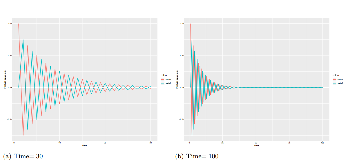
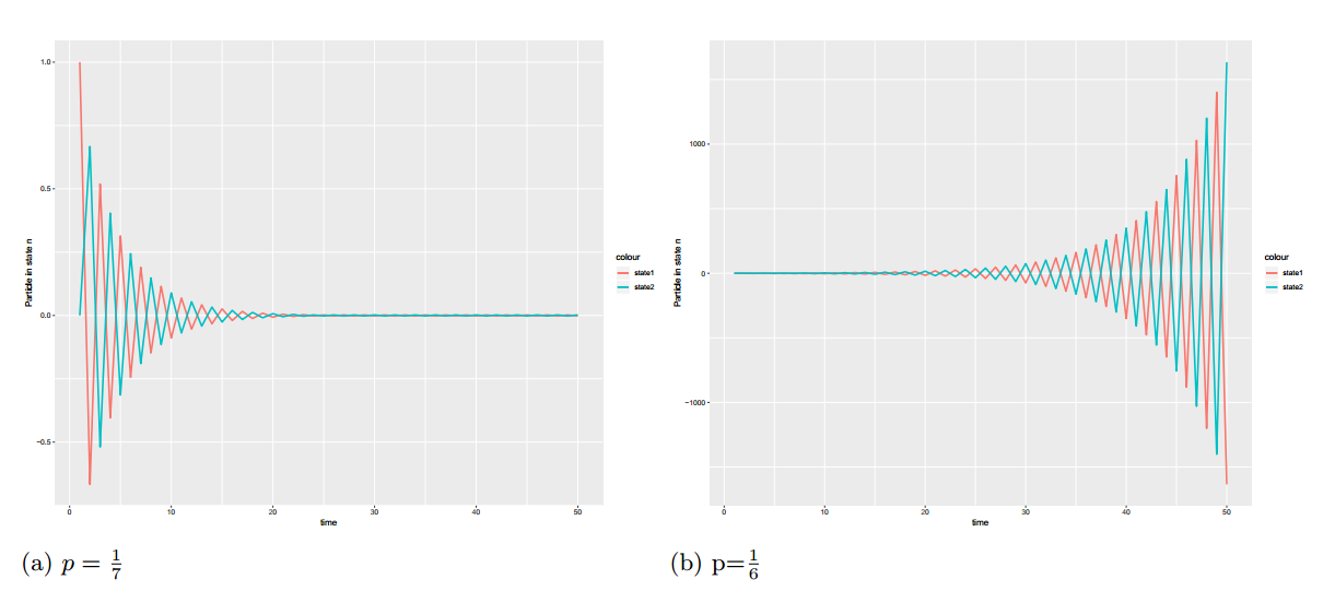
Figure 7 and Figure 8 plot the impact of the probability and the time on the attainment of the equilibrium in a hexagonal tiling when we consider continuous time.
Figure 7. Simulation of effect of variation of time on the attainment of the equilibrium for fixed probability(transition rate \(\alpha=\frac{1}{8}\))Figure 8. Simulation of effect of variation of probability on the attainment of the equilibrium for fixed time
The collection of graphs illustrated on Figure 7 and Figure 8 depicts how fast the molecule reaches the equilibrium in the hexagonal tiling in continuous time. The main factor which affects the attainment of the equilibrium is the transition rate. The transition rate \(\alpha=\frac{1}{6}\) is a critical value which affects particularly the motion of the molecule in the hexagonal tiling. For this value, if the molecule quits the central cell, it will never come back into it. A quick substitution in Equation (35) and a glance on Figure 8b can allow to verify it.
5. Discussion of results and conclusion
Under continuous-time conditions, we have checked the same results. In fact, Equation (30) and Equation (35) show that the average transition time from state 1 to state 2 is greater in the square tiling than in the hexagonal tiling. A glance at the panels of graphs depicted above shows that the greater the probability (transition rate), the later the equilibrium is reached in both square and hexagonal tilings. However, when comparing the movement in both tilings, we realize that the equilibrium is quickly reached in hexagonal tiling than in the square one. Increasing the value of the transition rate leads to a quick or late attainment of the equilibrium.
In this paper, the movement of a molecule in two kinds of tilings has been studied: the square tiling and the hexagonal one. Its has been established that only two parameters, among the four considered, have an impact on the quick or late attainment of the equilibrium. The parameters under consideration in this study were the nature of the time (discrete or continuous), the probability (so called transition rate), the time and the shape of the tiling.
In [1], the movements of the molecules in the tilings were modelled using discrete-time Markov chains. It was established that this motion reaches the equilibrium point faster in the hexagonal tiling than in the square one. This same finding is established in continuous-time Markov chains. It is to be deduced that the nature of time does not have an impact on reaching the equilibrium point.However, the shape of the tiling is a core parameter for the attainment of the equilibrium. That is, the molecule is faster in hexagonal tiling than in the square one.
Another important parameter is the transition rate in the infinitesimal generator. During this study, it has been demonstrated that for both hexagonal and square tilings, the rapidity to attain the equilibrium depends also upon the transition rate under consideration. Hence, the smaller the transition rate, the faster the molecule is, in reaching the equilibrium position and vice versa. To put it in a nutshell, this study has proven the influence of transition rate and the shape of the tiling were important for the rapidity of the movement. Other parameters do not have considerable impact on the movement.
Author Contributions
All authors contributed equally to the writing of this paper. All authors read and approved the
final manuscript.
Competing Interests
The author(s) do not have any competing interests in the manuscript.
References
Saiguran, M., Ring, A., & Ibrahim, A. (2019). Evaluation of Markov chains to describe movements on tiling. Open Journal of Mathematical Sciences, 3(1), 358-381.[Google Scholor]
Brémaud, P. (2009). Initiation aux Probabilités: et aux chaînes de Markov. Springer Science & Business Media.[Google Scholor]
Ring, A. (2004). State symmetries in matrices and vectors on finite state spaces. arXiv preprint math/0409264.[Google Scholor]
Barr, D. R., & Thomas, M. U. (1977). An eigenvector condition for Markov chain lumpability. Operations Research, 25(6), 1028-1031.[Google Scholor]
Benec, V. E. (1978). Reduction of network states under symmetries. Bell System Technical Journal, 57(1), 111-149.[Google Scholor]
Nagle, R. K., Saff, E. B., Snider, A. D., & West, B. (1996). Fundamentals of differential equations and boundary value problems. Reading: Addison-Wesley, Pearson.[Google Scholor]
Whitt, W. (2013). Continuous-time Markov chains. Department of Industrial Engineering and Operations Research, Columbia University, New York, December 2013.[Google Scholor]
Kemeny, J. G., & Snell, J. L. (1976). Finite markov chains. Undergraduate Texts in Mathematics.[Google Scholor]
Tian, J. P., & Kannan, D. (2006). Lumpability and commutativity of Markov processes. Stochastic analysis and Applications, 24(3), 685-702.[Google Scholor]
Yin, G. G., & Zhang, Q. (2012). Continuous-time Markov chains and applications: a two-time-scale approach (Vol. 37). Springer Science & Business Media, New York.[Google Scholor]
Cameron, M., & Gan, T. (2016). A graph-algorithmic approach for the study of metastability in markov chains. arXiv preprint arXiv:1607.00078.[Google Scholor]
Meyn, S. P., & Tweedie, R. L. (2012). Markov chains and stochastic stability. Springer Science & Business Media.[Google Scholor]
Levin, D. A., & Peres, Y. (2017). Markov chains and mixing times (Vol. 107). American Mathematical Socity.[Google Scholor]
Schuette, C., & Metzner, P. (2009). Markov chains and Jump Processes. An Introduction to Markov and Jump Processes on Countable States Spaces. Freie Universit Berlin, Berlin.[Google Scholor]