In this paper, the reduced differential transform method (RDTM) is applied to solve fuzzy nonlinear partial differential equations (PDEs). The solutions are considered as infinite series expansions which converge rapidly to the solutions. Some examples are solved to illustrate the proposed method.
The fuzzy sets were introduced for the first time by Zadeh in [1]. Hundreds of examples have been supplied where the nature of uncertainty in the behavior of given system processes is fuzzy rather than stochastic nature. Recently, many authors showed interest in the study of the theoretical framework of fuzzy initial value problems. Chang and Zadeh [2] introduced the concept of fuzzy derivative. Dubosi and Prade [3] presented the extension principle. The differential and integral calculus for fuzzy-set-valued functions, shortly fuzzy-valued functions was developed in resent work, see [4,5,6,7,8,9].
It is known that phenomena of nature or physical systems can be modeled using partial differential equations (PDEs) such as wave equations, heat equations, Poisson’s equation and so on. Hence, studies of PDEs become one of the main topics of modern mathematical analysis and attracted much attention. Many authors developed different methods for solving different kinds of PDEs, see [10,11,12,13,14,15,16,17].
The differential transform method (DTM) was introduced by Zhou [18] and he applied it to solve initial value problems for electric circuit analysis. The DTM is based on Taylor,s series expansion and can be applied to solve both linear and nonlinear ordinary differential equations as well as PDEs.
Keskin and Oturanc [19] proposed the RDTM, defining a set of transformation rules to overcome the complicated complex calculations of traditional DTM. Recently some researchers used RDTM for solving different equations, see [20,21,22,23,24,25,26].
This paper is structured as follows: In Section 2, we call some definition on a fuzzy number, fuzzy-valued function and strongly generalized Hukuhara differentiability. In Section 3, Taylor’s formula, one-dimensional DTM, and two-and three-dimensional RDTM is introduced. In Section 4, we provide some examples to show the efficiency and simplicity of RDTM. Finally, Section 5 consists of some brief conclusions.
2. Basic concepts
The fuzzy set \(\tilde{u}\in E^{1}\) is called a fuzzy number if \(\tilde{u}\) is a normal, convex fuzzy set, upper semi-continuous and supp\(u=\{x\in R|u(x)>0\}\) is compact. Here \(\overline{A}\) denotes the closure of \(A.\) We use \(E^{1}\) to denote the fuzzy number space [27,28].
For \(\tilde{u},\tilde{v}\in E^{1}\), \(k\in R\), the addition and scalar multiplication are defined by
\begin{align}
[\tilde{u}+\tilde{v}]_{r}&=[\tilde{u}]_{r}+[\tilde{v}]_{r},\nonumber\\
[k\tilde{u}]_{r}&=k[\tilde{u}]_{r},\nonumber
\end{align}
respectively, where \([\tilde{u}]_{r}=\{x:u(x)\geq r\}=[\underline{u}_{r},\overline{u}_{r}]\) for any \(r\in[0,1]\).
We use the Hausdorff distance between fuzzy numbers [28] \(D:E^{1}\times E^{1}\rightarrow[0,+\infty)\) defined by
\begin{align}
D(\tilde{u}+\tilde{v})&=\sup_{r\in[0,1]}d([\tilde{u}]_{r}[\tilde{v}]_{r})\nonumber\\
&=\sup_{r\in[0,1]}\max\{|\underline{u}_{r}-\underline{v}_{r}|,|\overline{u}_{r}
-\overline{v}_{r}|\},\nonumber
\end{align}
where \(d\) is the Hausdorff metric. \(D(\tilde{u},\tilde{v})\) is called the distance between \(\tilde{u}\) and \(\tilde{v}\).
Definition 1. [29,30] Let \(\tilde{u}\) be a fuzzy number defined in \({F(R)}\). The \(r\)-level set of \(\tilde{u}\), for any \(r\in[0,1]\) denoted by \(\tilde{u}_{r}\) is a crisp set that contains all elements in \(R\), such that the membership value of \(\tilde{u}\) is greater or equal to \(r\), that is
\[
\tilde{u}_{r}=\{{x\in R|\tilde{u}(x)\geq r}\}.
\]
Whenever we represent the fuzzy number with \(r\)-level set, we mean that it is closed and bounded and it is denoted by \([\underline{u}_{r},\overline{u}_{r}]\), where they represent the lower and upper bound \(r\)-level set of a fuzzy number.
The researchers [31,32] defined the parametrical representation of the fuzzy numbers as in the following definition:
Definition 2. [33] A fuzzy number \(\tilde{u}\) in parametric form is a pair \([\underline{u}_{r},\overline{u}_{r}]\) of functions \(\underline{u}_{r}\) and \(\overline{u}_{r}\) for any \(r\in[0,1]\), which satisfies the following requirements
\(\underline{u}_{r}\) is a bounded non-decreasing left continuous function in (0,1];
\(\overline{u}_{r}\) is a bounded non-increasing left continuous function in (0,1];
\(\underline{u}_{r}\leq\overline{u}_{r}.\)
Some researchers classified the fuzzy numbers into several types of the fuzzy membership function and the triangular fuzzy membership function or also often referred to as triangular fuzzy number is the most widely used membership function.
In order to avoid the inconvenience, in the whole paper, the fuzzy numbers and fuzzy-valued functions are represented with a tilde sign at the top, while the real-value function and interval-valued functions are written directly.
Definition 3. [34] A fuzzy valued function \(\tilde{f}\) of two variable is a rule that assigns to each ordered pair of real numbers, \((x,t)\), in a set \(D\), a unique fuzzy number denoted by \(\tilde{f}(x,t)\). The set \(D\) is the domain of \(\tilde{f}\) and its range is the set of values taken by \(\tilde{f}\), i.e., \(\{\tilde{f}(x,t)|(x,t)\in D\}\).
The parametric representation of the fuzzy valued function \(f:D\rightarrow E^{1}\) is expressed by \(\tilde{f}(x,t;r)=[\underline{f}(x,t;r),\overline{f}(x,t;r)]\), for all \((x,t)\in D\) and \(\alpha\in[0,1]\).
Definition 4. [34,35] A fuzzy valued function \(f:D\rightarrow E^{1}\) is said to be fuzzy continuous at \((x_{0},t_{0})\in D\) if \(\lim_{(x,t)\rightarrow(x_{0},t_{0})}\tilde{f}(x,t)=f(x_{0},t_{0})\). We say that \(\tilde{f}\) is fuzzy continuous on \(D\) if \(\tilde{f}\) is fuzzy continuous at every point \((x_{0},t_{0})\) in \(D\).
Definition 5. [36,37] The generalized Hukuhara difference of two fuzzy numbers \(\tilde{u},\tilde{v}\in E^{1}\) is defined as follows:
In terms of the \(r-\)levels, we get \([\tilde{u}\ominus_{gH}\tilde{v}]=[\min\{\underline{u}_{r}-
\underline{v}_{r},\overline{u}_{r}-\overline{v}_{r}\},\max\{\underline{u}_{r}
-\underline{v}_{r},\overline{u}_{r}-\overline{v}_{r}\}]\) and if the H-difference exists, then \(\tilde{u}\ominus\tilde{v}=\tilde{u}\ominus_{gH}\tilde{v}\); the conditions for existence of \(\tilde{w}=\tilde{u}\ominus_{gH}\tilde{v}\in E^{1}\) are
It is easy to show that (i) and (ii) are both valid if and only if \(\tilde{w}\) is a crisp number. In this case, it is possible that the gH-difference of two fuzzy numbers does not exist. To address this shortcoming, a new difference of fuzzy numbers was presented in [37]
Definition 6. [38] Let \(\tilde{u}(x,t): D\rightarrow E^{1}\) and \((x_{0},t)\in D\). We say that \(\tilde{u}\) is strongly generalized Hukuhara differentiable on \((x_{0},t)\) (gH-differentiable for short) if there exists an element \(\frac{\partial \tilde{u}}{\partial x}|_{(x_{0},t)}\in E^{1}\) such that
(i)   for all \(h>0\) sufficiently small, \(\exists\; \tilde{u}(x_{0}+h,t)\ominus_{gH} \tilde{u}(x_{0},t), \tilde{u}(x_{0},t) \ominus_{gH} \tilde{u}(x_{0}-h,t)\) and the limits (in the metric D)
\begin{equation}
\lim_{h\rightarrow0+}\frac{\tilde{u}(x_{0}+h,t)\ominus_{gH} \tilde{u}(x_{0},t)}{h}=\lim_{h\rightarrow0+}=\frac{ \tilde{u}(x_{0},t) \ominus_{gH} \tilde{u}(x_{0}-h,t)}{h}=\left.\frac{\partial \tilde{u}}{\partial x}_{_{gH}}\right|_{(x_{0},t)},\nonumber
\end{equation}
or
  (ii) for all \(h>0\) sufficiently small, \(\exists\; \tilde{u}(x_{0},t) \ominus_{gH} \tilde{u}(x_{0}+h,t), \tilde{u}(x_{0}-h,t)\ominus_{gH} \tilde{u}(x_{0},t)\) and the limits
\begin{equation}
\lim_{h\rightarrow0+}\frac{\tilde{u}(x_{0},t)\ominus_{gH} \tilde{u}(x_{0}+h,t)}{-h}
=\lim_{h\rightarrow0+}\frac{\tilde{u}(x_{0}-h,t)\ominus_{gH} \tilde{u}(x_{0},t)}{-h}=\left.\frac{\partial \tilde{u}}{\partial x}_{gH}\right|_{(x_{0},t)},\nonumber
\end{equation}
or
(iii)   for all \(h>0\) sufficiently small, \(\exists\; \tilde{u}(x_{0}+h,t)\ominus_{gH} \tilde{u}(x_{0},t), \tilde{u}(x_{0}-h,t)\ominus_{gH} \tilde{u}(x_{0},t)\) and the limits
\begin{equation}
\lim_{h\rightarrow0+}\frac{\tilde{u}(x_{0}+h,t)\ominus_{gH} \tilde{u}(x_{0},t)}{h}=\lim_{h\rightarrow0+}\frac{\tilde{u}(x_{0}-h,t)\ominus_{gH} \tilde{u}(x_{0},t)}{-h}=\left.\frac{\partial \tilde{u}}{\partial x}_{gH}\right|_{(x_{0},t)},\nonumber
\end{equation}
or
(iv)   for all \(h>0\) sufficiently small, \(\exists\; \tilde{u}(x_{0},t) \ominus_{gH} \tilde{u}(x_{0}+h,t), \tilde{u}(x_{0},t) \ominus_{gH} \tilde{u}(x_{0}-h,t)\) and the limits
\begin{equation}
\lim_{h\rightarrow0+}\frac{\tilde{u}(x_{0},t)\ominus_{gH} \tilde{u}(x_{0}+h,t)}{-h}=\lim_{h\rightarrow0+}\frac{ \tilde{u}(x_{0},t) \ominus_{gH} \tilde{u}(x_{0}-h,t)}{h}=\left.\frac{\partial \tilde{u}}{\partial x}_{gH}\right|_{(x_{0},t)}.\nonumber
\end{equation}
Lemma 1. [39] Let \(\tilde{u}(x,t):
D \rightarrow E^1.\) Then the following statements hold:
(a)   If \(\tilde{u}(x,t)\) is \((i)\)-partial differentiable for \(x\) (i.e., \(\tilde{u}\) is partial differentiable for \(x\) under the meaning of Definition 5 \((i)\), similarly to \(t\)), then
(b)   If \(\tilde{u}(x,t)\) is \((ii)\)-partial differentiable for \(x\) (i.e., \(\tilde{u}\) is partial differentiable for \(x\) under the meaning of Definition 5 \((ii)\), similarly to \(t\)), then
Theorem 1. If the function \(f(x)\) has \((n+1)\) derivatives on an interval \((c-r,c+r)\) for some \(r>0\), and \(\lim_{n\rightarrow\infty}R_{n}(x)=0\), for all \(x\in(c-r,c+r)\), where \(R_{n}(x)\) is the error between \(F_{n}(x)\) and the polynomial function \(f(x)\) then the Taylor series expanded about \(x=c\) converges to \(f(x).\) Thus
The Equation (9) is the Taylor series expansion of \(f(x)\) at \(x=x_{0}\). From Equations (10) and (11), the following basic operations of DTM can be deduced
  If \(f(x)=y_{1}(x)\pm y_{2}(x),~~\mbox {then}~~ F(j)=Y_{1}(j)\pm Y_{2}(j).\)
  If \(f(x)=ay_{1}(x), ~\mbox {then}~~ F(j)=aY_{1}(j), \mbox{where a is a constant}.\)
  If \(f(x)=\frac{dy_{1}(x)}{dx}~~\mbox {then}~~F(j)=(j+1)Y_{1}(j+1)\).
  If \(f(x)=\frac{d^{2}y_{1}(x)}{dx^{2}}~~\mbox {then}~~F(j)=(j+1)(j+2)Y_{1}(j+2)\).
  If \(f(x)=\frac{d^{n}y_{1}(x)}{dx^{n}},~~\mbox {then}~~ F(j)=\frac{(j+1)!}{j!}Y_{1}(j+1).\)
  If \(f(x)=y_{1}(x)y_{2}(x),~~\mbox {then}~~ F(x)=\sum^{j}_{i=0}Y_{1}(i)Y_{2}(j-i).\)
  If \(f(x)=x^{n},~~\mbox {then}~~ F(j)=\mu(j-n)~~\mbox where ~\mu(j-n) =\left\{\begin{aligned}
&1, ~~~j=n,\\
&0, ~~~j\neq n.
\end{aligned}\right.\)
  If \(f(x)=(1+x)^{n}~~\mbox {then}~~F(j)=\frac{n(n-1)……(n-j+1)}{j!}\).
  If \(f(x)=e^{a x},~~\mbox {then}~~ F(j)=\frac{a^{j}}{j!},\mbox {where \(a\) is a constants}.\)
  If \(f(x)=\sin(\omega x+\alpha),\mbox {then}~ F(j)=\frac{\omega^{j}}{j!}\sin(\frac{j\pi}{2}+\alpha),~\mbox{ where \(\omega\) and \(\alpha\) are constants}.\)
  If \(f(x)=cos(\omega x+\alpha), \mbox {then} F(j)=\frac{\omega^{j}}{j!}\cos(\frac{j\pi}{2}+\alpha),~\mbox{ where \(\omega\) and \(\alpha\) are constants}.\)
3.2. Reduced differential transform method
We consider the following two-dimensional RDTM:
Definition 10. [41] If the function \(w(x,t)\) is analytical and differentiable continuously with respect to time \(t\) and space \(x\) in the domain of interest, then we get
where the t-dimensional spectrum function \(W_{j}(x)\) is the transformed function of \(w(x,t)\). Here the lower case function \(w(x,t)\) represents the original function while the upper case \(W_{j}(x)\) stands for the transformed function.
Definition 11. [41] The inverse differential transform of \(W_{j}(x)\) is defined as
for \(r\in [0,1],\) where \(\underline{u}\) stands for \(\underline{u}(x,t;r),\) and \(\overline{u}\) stands for \(\overline{u}(x,t;r).\)
Applying the RDTM on Equations (18) and (19), we get the recurrence relation as
Substituting \(\tilde{U}_{0}(x;r) = [\underline{U}_{0}(x;r), \overline{U}_{0}(x;r)]\) into the recurrence relation (20), we get the following \(\tilde{U}_{j}(x;r)\) values successively
\begin{align}
\left.\begin{aligned}
\underline{U}_{1}(x;r)&=2(x^{2}+5)r^{n}\nonumber\\
\underline{U}_{2}(x;r)&=\frac{2^{2}(x^{2}+5)r^{n}}{2!}\nonumber\\
\overline{U}_{3}(x;r)&=\frac{2^{3}(x^{2}+5)r^{n}}{3!}\nonumber\\
\overline{U}_{4}(x;r)&=\frac{2^{4}(x^{2}+5)r^{n}}{4!}\nonumber\\
\vdots\nonumber
\end{aligned}\right\}
\end{align}
and
\begin{align}
\left.\begin{aligned}
\underline{U}_{1}(x;r)&=2(x^{2}+5)(2-r)^{n}\nonumber\\
\underline{U}_{2}(x;r)&=\frac{2^{2}(x^{2}+5)(2-r)^{n}}{2!}\nonumber\\
\overline{U}_{3}(x;r)&=\frac{2^{3}(x^{2}+5)(2-r)^{n}}{3!}\nonumber\\
\overline{U}_{4}(x;r)&=\frac{2^{4}(x^{2}+5)(2-r)^{n}}{4!}\nonumber\\
\vdots\nonumber
\end{aligned}\right\}
\end{align}
The inverse differential transform of \(\tilde{U}_{j}(x;r)\) is obtained from the relations
\begin{align}
\underline{u}(x,t;r)&=\sum^{\infty}_{j=0}\underline{U}_{j}(x;r)t^{j},\nonumber\\
\overline{u}(x,t;r)&=\sum^{\infty}_{j=0}\overline{U}_{j}(x;r)t^{j},\nonumber
\end{align}
and the exact solution is
\begin{align}
\tilde{u}(x,t;r)&=\left[r^{n},(2-r)^{n}\right]\odot\left((x^{2}+5)e^{2t}+x-5\right), \;\;\;\; 0\leq r\leq1.\nonumber
\end{align}
Example 2. Consider the following two-dimensional initial value problem describing fuzzy heat-like equations
for \(r\in [0,1],\) where \(\underline{u}\) stands for \(\underline{u}(x,t)(r)\) and \(\overline{u}\) stands for \(\overline{u}(x,t)(r),.\)
Applying the RDTM on Equations (26) and (27), we get the recurrence relation as
where \(\tilde{U}_{j}(x,y;r)\) is the transform function. From the initial condition (24), we get
\begin{align*}
\underline{U}_{0}(x,y;r)&=(0.2+0.2r)^{n}+(x^{2}+y^{2}),\\
\overline{U}_{0}(x,y;r) &=(0.6-0.2r)^{n}+(x^{2}+y^{2}).
\end{align*}
Substituting \(\tilde{U}_{0}(x,y;r)\) into the recurrence relation (28), we get the following \(\tilde{U}_{j}(x,y;r)\) values successively
\begin{align}
\left.\begin{aligned}
\underline{U}_{1}(x,y;r)&=(0.2+0.2r)^{n}+(x^{2}+y^{2})\nonumber\\
\underline{U}_{2}(x,y;r)&=\frac{(0.2+0.2r)^{n}+(x^{2}+y^{2})}{2!}\nonumber\\
\underline{U}_{3}(x,y;r)&=\frac{(0.2+0.2r)^{n}+(x^{2}+y^{2})}{3!}\nonumber\\
\underline{U}_{4}(x,y;r)&=\frac{(0.2+0.2r)^{n}+(x^{2}+y^{2})}{4!}\nonumber\\
\vdots\nonumber
\end{aligned}\right\}
\end{align}
and
\begin{align}
\left.\begin{aligned}
\overline{U}_{1}(x,y;r)&=(0.6-0.2r)^{n}+(x^{2}+y^{2})\nonumber\\
\overline{U}_{2}(x,y;r)&=\frac{(0.6-0.2r)^{n}+(x^{2}+y^{2})}{2!}\nonumber\\
\overline{U}_{3}(x,y;r)&=\frac{(0.6-0.2r)^{n}+(x^{2}+y^{2})}{3!}\nonumber\\
\overline{U}_{4}(x,y;r)&=\frac{(0.6-0.2r)^{n}+(x^{2}+y^{2})}{4!}\nonumber\\
\vdots\nonumber
\end{aligned}\right\}
\end{align}
The solution for \(\tilde{u}(x,t;r)\) is
\begin{align}
\underline{u}(x,y,t;r)&=\sum^{\infty}_{j=0}\underline{U}_{j}(x,y;r)t^{j}=(0.2+0.2r)^{n}+\left[(x^{2}+y^{2})\left(1+t+\frac{t^{2}}{2!}+\frac{t^{3}}{3!}
+\frac{t^{4}}{4!}+\cdot\cdot\cdot\infty\right)\right],\nonumber\\
\overline{u}(x,y,t;r)&=\sum^{\infty}_{j=0}\overline{U}_{j}(x,y;r)t^{j}=(0.6-0.2r)^{n}+\left[(x^{2}+y^{2})\left(1+t+\frac{t^{2}}{2!}+\frac{t^{3}}{3!}
+\frac{t^{4}}{4!}+\cdot\cdot\cdot\infty\right)\right],\nonumber
\end{align}
and the exact solution is
\begin{align}
\tilde{u}(x,y,t;r)=\left[(0.2+0.2r)^{n},(0.6-0.2r)^{n}\right]\oplus\left((x^{2}+y^{2})\exp(t)\right), 0\leq r\leq 1.\nonumber
\end{align}
Example 3. We consider following two-dimensional initial value problem describing heat-like equations
where \(\delta(j) = 1\) when \(j = 0\), and \(\delta(j) = 0\) when \(j\neq0\). Moreover \(\tilde{U}_{j}(x,y;r) = \left[\underline{U}_{j}(x,y;r), \overline{U}_{j}(x,y;r)\right]\) is the transform function. From the initial conditions, we obtain
for \(r\in [0,1],\) where \(\underline{u}\) stands for \(\underline{u}(x,t)(r)\) and \(\overline{u}\) stands for \(\overline{u}(x,t)(r)\).
Applying the RDTM on Equations (37) and (38), we get the recurrence relation as
For different values of \(j\), we get the following results
\begin{align}
\left.\begin{aligned}
\underline{U}_{1}(x;r)&=(0.5+0.5r)-1\nonumber\\
\underline{U}_{2}(x;r)&=(0.5+0.5r)+1\nonumber\\
\underline{U}_{3}(x;r)&=(0.5+0.5r)-1\nonumber\\
\underline{U}_{4}(x;r)&=(0.5+0.5r)+1\nonumber\\
\vdots\nonumber
\end{aligned}\right\}
\end{align}
and
\begin{align}
\left.\begin{aligned}
\overline{U}_{1}(x;r)&=(1.5-0.5r)-1\nonumber\\
\overline{U}_{2}(x;r)&=(1.5-0.5r)+1\nonumber\\
\overline{U}_{3}(x;r)&=(1.5-0.5r)-1\nonumber\\
\overline{U}_{4}(x;r)&=(1.5-0.5r)+1\nonumber\\
\vdots\nonumber
\end{aligned}\right\}
\end{align}
The solution for \(\tilde{u}(x,t;r)\) is
\begin{align}
\underline{u}(x,t;r)&=\sum^{\infty}_{j=0}\underline{U}_{j}(x;r)t^{j}
= \left(\underline{U}_{0}(x;r)+\underline{U}_{1}(x;r)t+\underline{U}_{2}(x;r)t^{2}+
\underline{U}_{3}(x;r)t^{3}+\cdot\cdot\cdot\right)\nonumber\\
&=(0.5+0.5r)+(1-t+t^{2}-t^{3}+\cdot\cdot\cdot),\nonumber\\
\overline{u}(x,t;r)&=\sum^{\infty}_{j=0}\overline{U}_{j}(x;r)t^{j}
= \left(\overline{U}_{0}(x;r)+\overline{U}_{1}(x;r)t+\overline{U}_{2}(x;r)t^{2}
+\overline{U}_{3}(x;r)t^{3}+\cdot\cdot\cdot\right)\nonumber\\
&=(1.5-0.5r)+(1-t+t^{2}-t^{3}+\cdot\cdot\cdot),\nonumber
\end{align}
and the exact solution is
\begin{align}
\tilde{u}(x,t;r) = \left[(0.5+0.5r)^{n},(1.5-0.5r)^{n}\right]\oplus\left[\frac{1}{1+t}\right],\;\;\; 0\leq r\leq 1.\nonumber
\end{align}
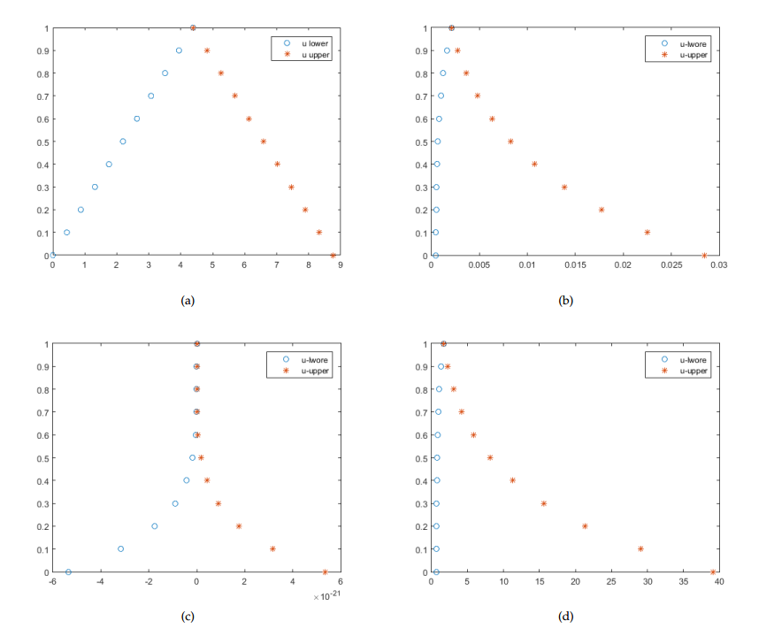
Figure 1 illustrate that the left-hand functions of the r-level set of \(\tilde{u}\) (u lower) are always increasing functions of \(r\) and the right-hand functions of the r-level set of \(\tilde{u}\) (u upper) are always decreasing functions of \(r\) in the above examples.
5. Conclusion
In this paper, the reduced differential transform method (RDTM) has been successfully applied for solving fuzzy nonlinear partial differential equations under gH-differentiability. The solutions are considered as infinite series expansions that converge rapidly to the exact solutions. We solved some examples to illustrate the proposed method. The results reveal that the proposed method is a powerful and efficient technique for solving fuzzy nonlinear partial differential equations.
Figure 1. \((a)\) Ex (4.1)\( x = 0.2,~ t = 0.3,~ n = 1.\) \((b)\) Ex (4.2)\( x = 0.0004,~y = 0.0005,~ t = 7,~ n = 7.\) \((c)\) Ex (4.3)\( x = 0.000002,~ y = 0.000003, t = 5,~ n = 5.\) \((d)\) Ex (4.4)\( t = 0.4,~ n = 9.\)
Author Contributions
All authors contributed equally to the writing of this paper. All authors read and approved the final manuscript.
Conflicts of Interest
The authors declare no conflict of interest.
References
Zaden, L. A. (1965). Fuzzy sets. lnformation and Control, 8, 338-353. [Google Scholor]
Chang, S. S., & Zadeh, L. A. (1996). On fuzzy mapping and control. In Fuzzy Sets, Fuzzy Logic, and Fuzzy Systems: selected papers by Lotfi A Zadeh (pp. 180-184). [Google Scholor]
Dubois, D., & Prade, H. (1982). Towards fuzzy differential calculus part 3: Differentiation. Fuzzy sets and Systems, 8(3), 225-233. [Google Scholor]
Dubois, D., & Prade, H. (1982). Towards fuzzy differential calculus part 1: Integration of fuzzy mappings. Fuzzy Sets and Systems, 8(1), 1-17. [Google Scholor]
Dubois, D., & Prade, H. (1982). Towards fuzzy differential calculus part 2: Integration on fuzzy intervals. Fuzzy Sets and Systems, 8(2), 105-116. [Google Scholor]
Dubois, D., & Prade, H. (1982). Towards fuzzy differential calculus part 3: Differentiation. Fuzzy Sets and Systems, 8(3), 225-233. [Google Scholor]
Puri, M. L., & Ralescu, D. A. (1983). Differentials of fuzzy functions. Journal of Mathematical Analysis and Applications, 91(2), 552-558. [Google Scholor]
Puri, M. L., & Ralescu, D. (1983). Differential of fuzzy functions. Journal of Mathematical Analysis and Applications, 91, 321-325. [Google Scholor]
Goetschel Jr, R., & Voxman, W. (1986). Elementary fuzzy calculus. Fuzzy Sets and Systems, 18(1), 31-43. [Google Scholor]
Kharab, A., & Kharab, R. (1997). Spreadsheet solution of hyperbolic partial differential equations [for EM field calculations]. IEEE Transactions on Education, 40(1), 103-110. [Google Scholor]
Kincaid, D., Kincaid, D. R., & Cheney, E. W. (2009). Numerical Analysis: Mathematics of Scientific Computing,(Vol. 2). American Mathematical Socity. [Google Scholor]
Biro, O., & Preis, K. (1990). Finite element analysis of 3-D eddy currents. IEEE Transactions on Magnetics, 26(2), 418-423. [Google Scholor]
McDonald, B. H., & Wexler, A. (1972). Finite-element solution of unbounded field problems. IEEE Transactions on Microwave Theory and Techniques, 20(12), 841-847.[Google Scholor]
Gratkowski, S., Pichon, L., & Razek, A. (1996). New infinite elements for a finite element analysis of 2D scattering problems. IEEE Transactions on Magnetics, 32(3), 882-885. [Google Scholor]
Osman, M., Gong, Z. T., & Mohammed, A. (2021). Differential transform method for solving fuzzy fractional wave equation. Journal of Computational Analysis and Applications, 29(3), 431-453.[Google Scholor]
Osman, M., Gong, Z., & Mustafa, A. M. (2020). Comparison of fuzzy Adomian decomposition method with fuzzy VIM for solving fuzzy heat-like and wave-like equations with variable coefficients. Advances in Difference Equations, 2020, Article No 327. [Google Scholor]
Osman, M., Gong, Z., & Mustafa, A. M. (2020). Applcation to the fuzzy fracrtional diffusion equation by using fuzzy fractional variational Homotopy pertubation iteration method. Advance Research Journal of Multidisciplinary Discoveries, 51(3), 15-26. [Google Scholor]
Zhou, J. K. (1986). Differential Transformation and its Application for Electcuits Circuits. Huarjung University press, Wuhan, China. [Google Scholor]
Keskin, Y., Servi, S., & Oturanç, G. (2011). Reduced differential transform method for solving Klein Gordon equations. In Proceedings of the World Congress on Engineering (Vol. 1, p. 2011). [Google Scholor]
Arshad, M., Lu, D., & Wang, J. (2017). (N+ 1)-dimensional fractional reduced differential transform method for fractional order partial differential equations. Communications in Nonlinear Science and Numerical Simulation, 48, 509-519. [Google Scholor]
Yu, J., Jing, J., Sun, Y., & Wu, S. (2016). \((n+1)-\)Dimensional reduced differential transform method for solving partial differential equations. Applied Mathematics and Computation, 273, 697-705. [Google Scholor]
Keskin, Y., & Oturanç, G. (2010). Application of reduced differential transformation method for solving gas dynamics equation. International Journal of Contemporary Mathematical Sciences, 22(22), 1091-1096. [Google Scholor]
Cenesiz, Y., Keskin, Y., & Kurnaz, A. (2010). The solution of the nonlinear dispersive \(K(m,n)\) equations by RDT method. International Journal of Nonlinear Science, 9,(4), 461-467. [Google Scholor]
Raslan, K. R., Biswas, A., & Sheer, Z. F. A. (2012). Differential transform method for solving partial differential equations with variable coefficients. International Journal of Physical Sciences, 7(9), 1412-1419. [Google Scholor]
Taha, B. A., & Abdul-Wahab, R. D. (2012). Numarical solutions of two-dimensional Burgers’ equations using reduced differential tranform method. Journal of Thi-Qar Science, 3(3), 252-264. [Google Scholor]
Neog, B. C. (2015). Solutions of some system of non-linear PDEs using reduced differential transform method. IOSR Journal of Mathematics, 11(5), 37-44. [Google Scholor]
Gong, Z., & Wang, L. (2012). The Henstock–Stieltjes integral for fuzzy-number-valued functions. Information Sciences, 188, 276-297. [Google Scholor]
Kaleva, O. (2006). A note on fuzzy differential equations. Nonlinear Analysis: Theory, Methods & Applications, 64(5), 895-900. [Google Scholor]
Kaleva, O. (1987). Fuzzy differential equations. Fuzzy Sets and Systems, 24(3), 301-317. [Google Scholor]
Ma, M., Friedman, M., & Kandel, A. (1999). Numerical solutions of fuzzy differential equations. Fuzzy Sets and Systems, 105(1), 133-138. [Google Scholor]
Friedman, M., Ma, M., & Kandel, A. (1999). Numerical solutions of fuzzy differential and integral equations. Fuzzy Sets and Systems, 106(1), 35-48. [Google Scholor]
Rahman, N. A. A., & Ahmad, M. Z. (2017). Solving fuzzy fractional differential equations using fuzzy Sumudu transform. Journal of Nonlinear Sciences and Applications, 10(5), 2620-2632.[Google Scholor]
Allahviranloo, T., Gouyandeh, Z., Armand, A., & Hasanoglu, A. (2015). On fuzzy solutions for heat equation based on generalized Hukuhara differentiability. Fuzzy Sets and Systems, 265, 1-23. [Google Scholor]
Guang-Quan, Z. (1991). Fuzzy continuous function and its properties. Fuzzy Sets and Systems, 43(2), 159-171. [Google Scholor]
Yang, H., & Gong, Z. (2019). Ill-posedness for fuzzy Fredholm integral equations of the first kind and regularization methods. Fuzzy Sets and Systems, 358, 132-149. [Google Scholor]
Bede, B., & Stefanini, L. (2013). Generalized differentiability of fuzzy-valued functions. Fuzzy Sets and Systems, 230, 119-141. [Google Scholor]
Bede, B., & Gal, S. G. (2005). Generalizations of the differentiability of fuzzy-number-valued functions with applications to fuzzy differential equations. Fuzzy Sets and Systems, 151(3), 581-599. [Google Scholor]
Chalco-Cano, Y., & Roman-Flores, H. (2008). On new solutions of fuzzy differential equations. Chaos, Solitons & Fractals, 38(1), 112-119. [Google Scholor]
Neog, B. C. (2015). Solutions of some system of non-linear PDEs using reduced differential transform method. IOSR Journal of Mathematics, 11(5), 37-44. [Google Scholor]
Keskin, Y., & Oturanc, G. (2009). Reduced differential transform method for partial differential equations. International Journal of Nonlinear Sciences and Numerical Simulation, 10(6), 741-750. [Google Scholor]
Mustafa, A. M., Gong, Z., & Osman, M. (2020). The solution of fuzzy variational problem and fuzzy optimal control problem under granular differentiability concept. International Journal of Computer Mathematics, https://doi.org/10.1080/00207160.2020.1823974.[Google Scholor]