
Vito Volterra in 1926 introduced integro-differential for the first time when he investigated the population growth, focussing his study on the hereditary influences, whereby through his research work the topic of integro-differential equations was established [1]. Mathematical modeling of real life problems often result in functional equations such as differential, integral and integro-differential equations. Many mathematical formulation of physical phenomena reduced to integro-differential equations like fluid dynamics, control theory, biological models and chemical kinetics [1,2,3,4,5,6,7,8].
Linear Integro-Differential Equation (LIDE) is an important branch of modern mathematics and arises often in many applied areas which include engineering, mechanics, physics, chemistry, astronomy, biology, economics, potential theory and electrostatics [9].
A variational iteration method and trapezoidal rule by Saadati et al., [10] was used for solving LIDEs. Manafianheris [11] applied modified laplace Adomian decomposition method. Bashir and Sirajo [12] used finite difference Simpson’s approach on Fredholm Integro-differential equation and proved the error estimation of the method. In the work of Aruchunan and Sulaiman [2], a numerical solution of first order linear Fredholm integro-differential equations was obtained using conjugate gradient method. A reliable algorithm with application was presented by Alwaneh et al., [13]. Consider a linear Volterra integro-differential equation (LVIDE) of the form:
The main objective of this paper is to propose a combination of finite difference-Simpson’s approach (FDSM) to solve (LVIDE) (1) by transforming the problem into a system of linear algebraic equations. We used Maple software to obtained the numerical solution. Some examples are given to test the accuracy and efficiency of the method.
The paper has been organized as follows; In Section 2, we presented the derivation of the method. Error estimation of the scheme is proved in Section 3 and numerical results and discussions are provided in Section 4. Finally Section 5 conclude the paper.
Now using composite Simpson’s with \(N\) subintervals. The integral part of (1) is approximated as:
\begin{align*}%\label{eqn2} \nonumber\displaystyle{\int_{a}^{x}k(x,t)u(t)dt} \approx& \displaystyle{\frac{h}{3}}[k(x,t_{0})u(t_{0})+4(k(x,t_{1})u(t_{1})+…+k(x,t_{N-1})u(t_{N-1})) \\ &+2(k(x,t_{2})u(t_{2})+…+k(x,t_{N-2})u(t_{N-2}))+k(x,t_{N})u(t_{N})]\\%\label{eqn3} % \nonumber to remove numbering (before each equation) \approx&\displaystyle{\frac{h}{3}}[k(x,t_{0})u(t_{0})+4k(x,t_{1})u(t_{1})+2k(x,t_{2})u(t_{2})+…+2k(x,t_{N-2})u(t_{N-2})) \nonumber \\ &+4k(x,t_{N-1})u(t_{N-1})+k(x,t_{N})u(t_{N})]. \end{align*} By discritizing along \(x\) and taking \(u'(x_{i})=u’_{i}\), \(f(x_{i})=f_{i}\), \(k(x_{i},t_{i})=k_{ij},\) \(k(x_{i},t_{i})\) vanishes for \(t_{j}>x_{i}\) we haveUsing Equations (3) for \(i=1,2,…,N-1\) and (4) for \(i=N\), we can generate a systems of linear equations for \(u_{1},u_{2},…,u_{N}\), which can be represented in a matrix form as \( KU=W, \) where
\[K=\left( \begin{array}{cccccccccccc} A_{11} & 1 & 0 & 0 & … & 0 & 0 & 0 \\ A_{21}-1 & B_{22} & 1 & 0 & … & 0 & 0 & 0 \\ A_{31}-1 & B_{32}-1 & A_{33} & 1 & … & 0 & 0 & 0 \\ % A_{41}-1 & B_{42} & A_{43}-1 & 0 & … & 0 & 0& 0 \\ . & . & . & . & . & . & . & . \\ . & . & . & . & . & . & . & . \\ . & . & . & . & . & . & . & . \\ % A_{N-31} & B_{N-32} & A_{N-33} & B_{N-34} & … & B_{N-3N-2}-1 & A_{N-3N-1} & 0 \\ A_{N-21} & B_{N-22} & A_{N-23} & B_{N-24} & … & B_{N-2N-2} & 1 & 0 \\ A_{N-11} & B_{N-12} & A_{N-13} & B_{N-14} & … & B_{N-1N-2}-1 & A_{N-1N-1} & 1 \\ A_{N1} & B_{N2} & A_{N3} & B_{N4} & … & B_{NN-2}+1 & A_{NN-1}-4 & C_{NN}+3 \\ \end{array} \right),\] \(U=\left( \begin{array}{c} u_{1} \\ u_{2} \\ . \\ . \\ . \\ u_{N} \\ \end{array} \right),\) and \(W=\left( \begin{array}{c} 2hf_{1}+(\frac{2}{3}h^2k_{10})u_{0} \\ 2hf_{2}+\frac{2}{3}h^2k_{20}u_{0} \\ . \\ . \\ 2hf_{N-1}+\frac{2}{3}h^2k_{N-10}u_{0} \\ 2hf_{N}+\frac{2}{3}h^2k_{N0}u_{0} \\ \end{array} \right).\)Theorem 1. Suppose that \(\mu_{1}, \mu_{2}, \mu_{3}\in(a,b)\) such that the errors \(e_{1}\) of central difference, \(e_{2}\) of second backward difference approximation and \(e_{3}\) of Simpson’s rule respectively are given by \(\frac{h^{2}}{6}u^{(3)}(\mu_{1})\), \(\frac{h^{2}}{4}u^{(4)}(\mu_{3})\) and \(\frac{(x_{N}-a)}{180}h^{4}u^{(4)}(\mu_{2})\). Then the error estimation of approximate solution of linear Volterra integro-differential Equation (1) by the scheme (3) and (4) is \( {\displaystyle e^{*}}\leq\frac{5(x_{N}-a)^{2}}{12N^{2}}G.\)
Proof. From the problems of LVIDES (3) and (4), the exact solution for \(i=1,2,…,N-1\)
Subtracting (3) and (4) from (5) and (6), we obtained the error term as follow:
\begin{align*} e&=\left|\frac{h^{2}}{6}u^{(3)}(\mu_{1})+\frac{h^{2}}{4}u^{(4)}(\mu_{3})-\left(\frac{(x_{N}-a)}{180}h^{4}u^{(4)}(\mu_{2})+\frac{(x_{N}-a)}{180}h^{4}u^{(4)}(\mu_{2})\right)\right|,\\ &= \left|\frac{h^{2}}{6}u^{(3)}(\mu_{1})+\frac{h^{2}}{4}u^{(4)}(\mu_{3})-\frac{(x_{N}-a)}{90}h^{4}u^{(4)}(\mu_{2})\right|,\\ &\leq \left|\frac{h^{2}}{6}u^{(3)}(\mu_{1})+\frac{h^{2}}{4}u^{(4)}(\mu_{3})\right|,\\ &\leq \left|\frac{h^{2}}{6}G_{1}+\frac{h^{2}}{4}G_{2}\right|, \end{align*} after taking \(G_{1}=u^{(3)}(\mu_{1})\) and \(G_{2}=u^{(4)}(\mu_{3}).\)Now, if we let \(G=max\{G_{1}, G_{2}\}\) we have
\begin{eqnarray*} e&\leq \left|\frac{h^{2}}{6}G+\frac{h^{2}}{4}G\right|,\leq \left|\frac{5h^{2}}{12}G\right|. \end{eqnarray*} Substituting \({\displaystyle h=\frac{x_{N}-a}{N}}\), we get \begin{equation*} e^{*}\leq \left|\frac{5(x_{N}-a)^{2}}{12N^{2}}G\right|. \end{equation*} Hence the proposed scheme is of second order convergence.Example 1. Consider LVIDE equation:
| \(x\) | Exact solution | FDSM | REA[15] |
|---|---|---|---|
| 0.0625 | -0.9374599377 | -0.970285632 | -0.939313 |
| 0.125 | -0.8746843974 | -0.881205977 | -0.877167 |
| 0.1875 | -0.8114509330 | -0.848304304 | -0.816836 |
| 0.250 | -0.7475504439 | -0.760345075 | -0.752159 |
| 0.3125 | -0.6827862105 | -0.723778451 | -0.691295 |
| 0.375 | -0.6169729163 | -0.635854259 | -0.623507 |
| 0.43750 | -0.5499356617 | -0.595245125 | -0.561194 |
| 0.500 | -0.4815089580 | -0.506345938 | -0.489657 |
| 0.5625 | -0.4115357039 | -0.461405361 | -0.425194 |
| 0.6250 | -0.3398661420 | -0.370577838 | -0.349485 |
| 0.6875 | -0.2663567891 | -0.316674778 | -0.282077 |
| 0.750 | -0.1908693447 | -0.231335606 | -0.201611 |
| 0.8125 | -0.1132695669 | -0.165028649 | -0.130719 |
| 0.8750 | -0.0334261204 | -0.08294371 | -0.0451471 |
| 0.93750 | 0.0487906069 | -0.005464919 | -0.0299532 |
| 1 | 0.1335097231 | 0.075642841 | -0.121113 |
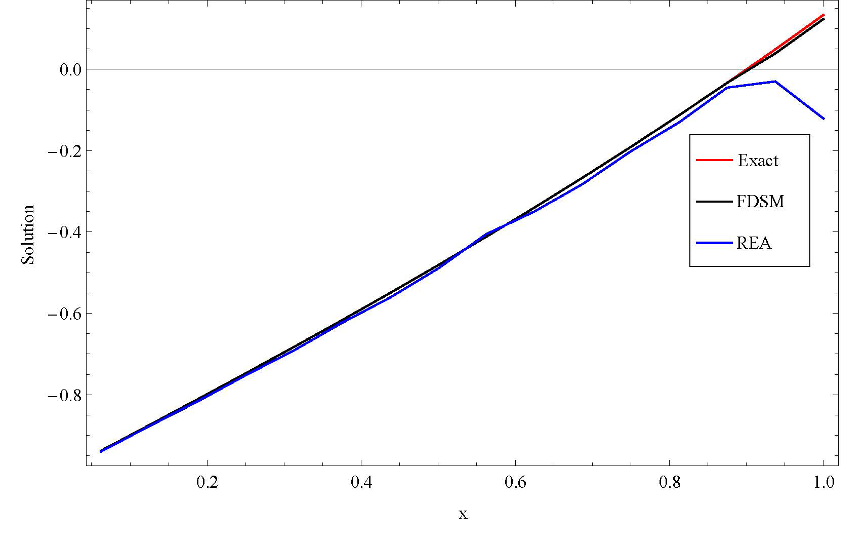
Table 1 shows the numerical results of Example 1. We compare the results obtained by using our method and numerical method of Romberg extrapolation algorithm (REA) given in [13]. Figure 1 indicate that our method of FDSM coincide with the exact solution and gives a better result than REA. This prove that our method is a good tool of approximating LVIDES problems of second kind.
Example 2. Consider LVIDE equation:
| \(x\) | Exact solution | FDSM | BVMs[17] |
|---|---|---|---|
| 0.1 | 0.7788007831 | 0.6913562245 | 0.5627307831 |
| 0.2 | 0.6065306597 | 0.5986143128 | 0.5781196597 |
| 0.3 | 0.4723665527 | 0.0467629062 | 0.4687287527 |
| 0.4 | 0.3678794412 | 0.3678699844 | 0.3674183412 |
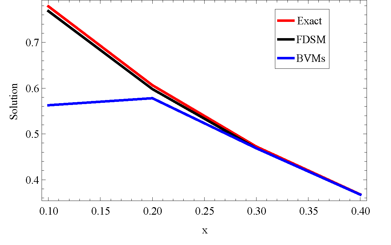
Table 2 shows the exact and the approximate solution obtained by our method at different values of \(x\) with the results of Boundary value methods (BVMs) given in [14]. Figure 2 provided a graphical presentation of the result which shows that our method can converge to the exact solution and gives a better result than BVMs.
Example 3. Consider LVIDE equation:
| \(x\) | Exact solution | FDSM | Absolute error |
|---|---|---|---|
| 0.1 | 0.09983341665 | 0.0966907300 | 3.143\(e-3\) |
| 0.2 | 0.1986693308 | 0.2009669073 | 2.298\(e-3\) |
| 0.3 | 0.2955202067 | 0.3006342060 | 5.114\(e-3\) |
| 0.4 | 0.3894183423 | 0.4099264019 | 2.051\(e-2\) |
| 0.5 | 0.4794255386 | 0.5166993051 | 3.727\(e-2\) |
| 0.6 | 0.5646424734 | 0.6352577593 | 7.061\(e-2\) |
| 0.7 | 0.6442176872 | 0.7535502344 | 1.093\(e-1\) |
| 0.8 | 0.7173560909 | 0.8859967676 | 1.686\(e-1\) |
| 0.9 | 0.7833269096 | 1.020684713 | 2.374\(e-1\) |
| 1 | 0.8414709848 | 1.172198061 | 3.307\(e-1\) |
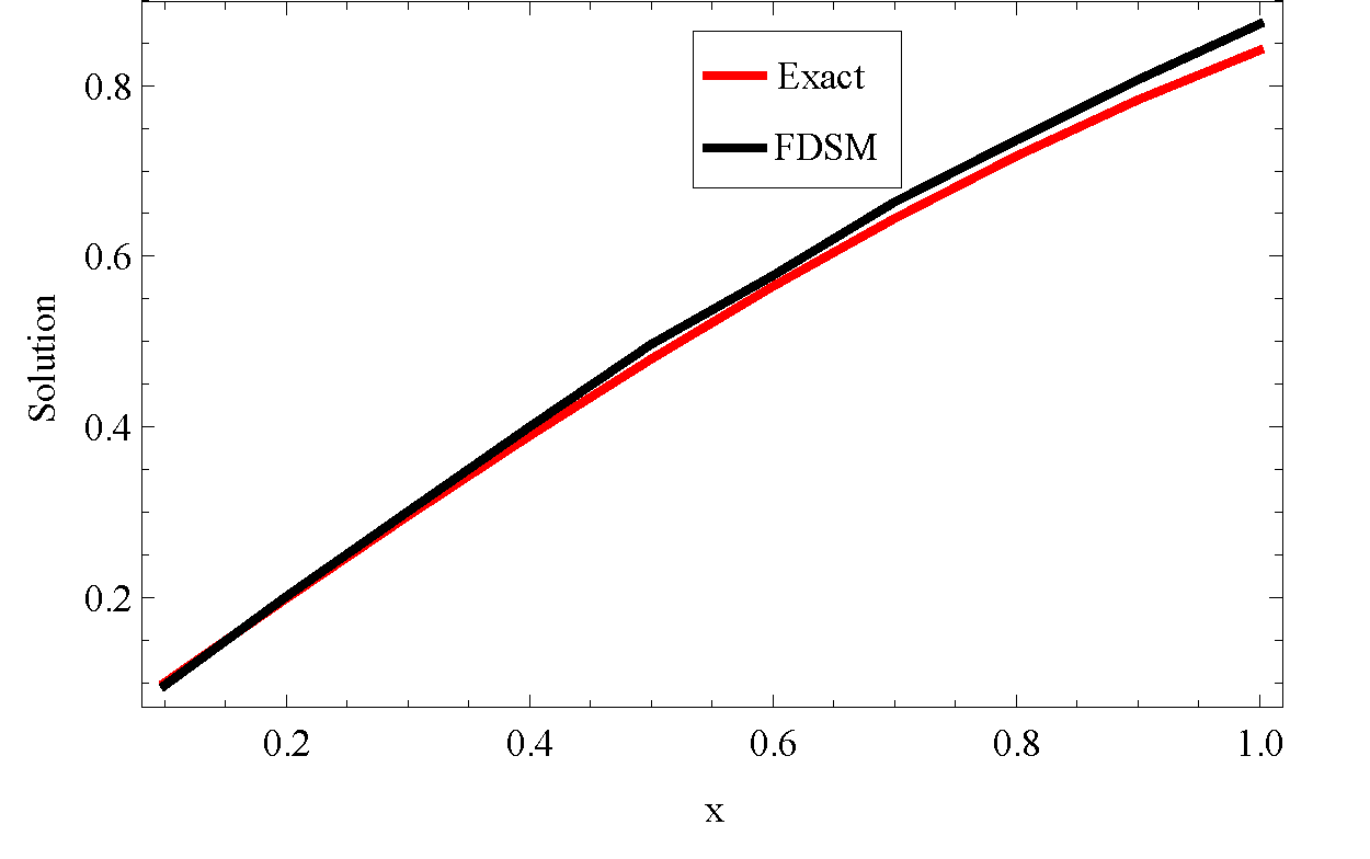
Table 3 shows the exact solution of the problem in Example 3 and the approximate solution obtained by our method. The absolute error obtained indicated that our method can give good approximation to LVIDE problems.