Open Journal of Mathematical Analysis

A simple two-strain HSV epidemic model with palliative treatment

Janet Kwakye, J. M. Tchuenche\(^1\)
Department of industrial Engineering, New Mexico State University, Las Cruces NM, USA.; (J.K)
School of Computational and Applied Mathematics, University of the Witwatersrand, Johannesburg, South Africa.; (J.M.T)
\(^{1}\)Corresponding Author: jmtchuenche@gmail.com

Abstract

A two-strain model of the transmission dynamics of herpes simplex virus (HSV) with treatment is formulated as a deterministic system of nonlinear ordinary differential equations. The model is then analyzed qualitatively, with numerical simulations provided to support the theoretical results. The basic reproduction number \(R_0\) is computed with \(R_0=\text{max}\lbrace R_1, R_2 \rbrace\) where \(R_1\) and \(R_2\) represent respectively the reproduction number for HSV1 and HSV2. We also compute the invasion reproductive numbers \(\tilde{R}_1\) for strain 1 when strain 2 is at endemic equilibrium and \(\tilde{R}_2\) for strain 2 when strain 1 is at endemic equilibrium. To determine the relative importance of model parameters to disease transmission, sensitivity analysis is carried out. The reproduction number is most sensitive respectively to the contact rates \(\beta_1\), \(\beta_2\) and the recruitment rate \(\pi\). Numerical simulations indicate the co-existence of the two strains, with HSV1 dominating but not driving out HSV2 whenever \(R_1 > R_2 > 1\) and vice versa.

Keywords:

Fixed point; Rectangular metric spaces; F-expansive mappings.

1. Introduction

Herpes simplex virus (HSV) is one of the most highly widespread sexually transmitted infections [1]. Lowestein confirmed the infectious nature of the HSV experimentally in 1919. In the years 1920s and 1930s, it was found that the HSV also infects the central nervous system [2]. The two strains of the disease are, HSV1 mostly known as cold sores and HSV2 also known as genital herpes. Both strains are transmitted sexually, however, HSV1 can also be transmitted non-sexually through contact with the fluid of an infected person. Looker et al., [3] estimated that about 417 million individuals with 267 million women inclusive age \(15-49\) have HSV2 infections worldwide, with the highest prevalence of 87% in Africa. Although South-East Asia and western pacific regions have a low prevalence of HSV2, they contribute significant amount to the global prevalence due to high population size. Fisman et al., [4] in their study on future dimensions and cost of HSV2 in the United States found that the prevalence of infection among individuals from age \(15-39\) years was projected to increase \(39%\) in men and \(49%\) in women by 2025.

In order to mitigate the spread and global socio-economic burden, mathematical modeling is an important tool that can provide insight into the long-term dynamics of a disease. It helps to simplify complex disease systems and has been a catalyst for decision making. Indeed, modeling has also been useful to present possible future outcomes of current trends and potential decision by policy makers. Some individuals infected with HSV are undiagnosed or do not display any physical symptoms. Latency is one of the major characteristics of the HSV [5,6,7]. Immunocompromised individuals with HSV stand a higher risk of acquiring HIV [8,9], and it has been found that HSV2 epidemics can more than double the peak of HIV incidence [8]. In fact, a key characteristic of HIV infection is poor control of herpes virus infections, which reactivate from latency and cause opportunistic infections in immunocompetent individuals [10].

Symptoms associated with HSV1 are tingling, itching or pains and sore throat which lead to blisters appearing on the face leading to sores, while in the case of HSV2, it appears on the genital areas [11,12] with associated symptoms such as headache, nerve pains, itching, lower abdominal pains, urinary difficulties, yeast infections, vaginal discharge, fever and open sores. Though HSV symptoms are mostly mild, there are other severity associated with such as ocular herpes which affects the eye leading to blindness; encephalitis also comes about as a result of being infected in the brain leading to death [13]. There is a reactivation after the latent infection to cause one or more rounds of the disease. And this reactivation can occur when infected individuals become sexually active again, weak immune system and inadequate or lack of treatment. Because there is currently neither complete treatment nor HSV vaccine, HSV which is a a life-long sexually-transmitted infection has no complete cure and an infected individual would live with it until death [14]. However, there are type-specific serology testing in the absence of symptoms which helps to determine the particular strain of the virus [15], and palliative treatment is administered to infected individuals to help get rid of the sores, reduce the risk of transmission as well as minimize the number and intensity of within host outbreaks. A study by the American College of Obstetricians and Gynecologists currently recommended the use of suppressive therapy to decrease transmission in discordant couples [16]. A comparison of two of these suppression drugs noted their effectiveness in decreasing both symptomatic and sub-clinical viral shedding [17,18].

Mathematical modeling is a useful tool to explore complex real life issue and guide experimental strategies and decision making [19]. Mathematical models of multiple strains of diseases such as HIV/AIDS, influenza and malaria have received much attention compared to HSV [20,21,22,23]. Nuno et al., [24] investigated the dynamics of a two-strain influenza with isolation and determined threshold conditions for the co-existence of the two strains. Because HSV treatement is only palliative, Schiffer et al., [25] developed a mathematical model to help optimize drug dose selection in clinical practice. To the best of our knowledge, a model that investigates conditions under which one strain of the virus would dominate or persist alone has not yet been considered. It is expected that this study will help fill the gap on HSV strains co-dynamics and provide a platform to further investigate if one strain could dominate and potentially drive the other to extinction.

The rest of this paper is organized as follows: The model formulation and the underlying assumptions are provided in \(§\)2. Theoretical analysis of the model is provided in \(§\)3. In \(§\)4, graphical representations generated (using the python programming language) to support the theoretical results are provided. \(§\)5 is the conclusion.

2. Model Formulation

Figure 1. The HSV epidemic model.

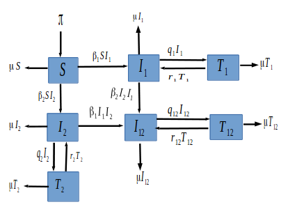
We formulate a simple HSV transmission dynamics model of the 2 HSV strains in the presence of treatment. Our model partitions the total population at any time \(t\) denoted by \( N(t)\) into seven epidemiological states depending on individuals disease status. The fully susceptible class denoted by \(S(t)\). The class of individuals who have come in contact with the HSV virus strain 1 and are infectious is denoted by \(I_{1}(t)\), and those in contact with the HSV2 virus and infectious is denoted by \(I_{2}(t)\). Individuals affected with the two strains are grouped in the \(I_{12}(t)\) class. The \(I_{1}(t)\) class of individuals who are on palliative treatment move to the \(T_1(t)\) class, and those in \(I_2(t)\) under palliative treatment move to the \(T_2(t)\) class. Individuals co-infected with both HSV1 and HSV2 strain \(I_{12}(t)\) under treatment move to the \(T_{12}(t)\) class.

Individuals are recruited into the susceptible compartment at a constant rate \(\pi\). Individuals in each compartment die naturally at a rate \(\mu\). Since there is no cure for HSV, treatment is just for relief and to reduce individual infectiousness. We assume no simultaneous infections by both strains. Susceptible individuals progress into \(I_{1}\) class at a transmission rate of \(\beta_1\) and to \(I_{2}\) class at a transmission rate of \(\beta_2\). Individuals in the \(I_{1}\) move to the \(T_{1}\) class and those in the \(I_{2}\) move to the \(T_{2}\) class at a treatment rate of \(q_{1}\) and \(q_{2}\) respectively or enter into the dual infection class at the rate of \(\beta_{2}\) and \(\beta_{1}\) respectively. The infected individuals with both diseases move to the \(T_{12}\) class at a rate of \(q_{12}\). Because treatment is not permanent, relapse is common, thus from the treatment class, the disease can re-activate at a rate \(r_{1}\), \(r_{2}\) and \(r_{12}\) into the \(I_{1}\), \(I_{2}\) and \(I_{12}\) class respectively. The description of the model variables and parameters are summarized in Table 1. Figure 1 gives a graphical interpretation of our proposed model based on the above description and assumptions.

Table 1. Description of model variables and parameters.
Description Value Reference
Parameter
\(\beta_1\) Transmission  rate  for individuals with HSV1 \(0.007(0.001-0.03)yr^{-1}\) Assumed
\(\beta_2\) Transmission  rate  for individuals with HSV2 \(0.001(0.001-0.03)yr^{-1}\) [26]
\(\mu\) natural death rate \(0.019(0.015-0.02)yr^{-1}\) [27]
\(r_1\) Reactivation  rate  of  HSV1 \(0.6\) Assumed
\(r_2\) Reactivation  rate  of  HSV2 \(0.6\) Assumed
\(r_{12}\) Reactivation  rate  of  both  HSV1 and HSV2 \(0.6\) Assumed
\(q_{12}\) Treatment     rate  of  both HSV1 and HSV2 \(0.45(0-1.0)yr^{-1}\) Assumed
\(q_{1}\) Treatment     rate  of  HSV1 \(0.45(0-1.0)yr^{-1}\) Assumed
\(q_{2}\) Treatment     rate  of  HSV2 \(0.45(0-1.0)yr^{-1}\) [28]
\(\pi\) Recruitment   rate \(0.3yr^{-1}\) Assumed
Variable
\(I_1(t)\) Individuals infected with HSV1
\(I_2(t)\) Individuals infected with HSV2
\(I_{12}(t)\) Individuals infected with both HSV1 and HSV2
\(T_1(t)\) Individuals infected with HSV1 and receiving treatment
\(T_2(t)\) Individuals infected with HSV2 and receiving treatment
\(T_{12}(t)\) Co-infected individuals receiving treatment

From the aforementioned, we established the following non-linear ordinary differential equations given by system (1)

\begin{eqnarray} \left. \begin{array}{rcl} \frac{dS}{dt}&=&\pi -\beta_{1}SI_{1}-\beta_{2}SI_{2}-\mu S,\\[5pt] \frac{dI_{1}}{dt}&=& \beta_{1}SI_{1}+r_{1}T_{1} -\beta_{2}I_{1}I_{2}-q_{1}I_{1}-\mu I_{1},\\[5pt] \frac{dI_{2}}{dt}&=& \beta_{2}SI_{2}+r_{2}T_{2} -\beta_{1}I_{2} I_{1}-q_{2}I_{2}-\mu I_{2},\\[5pt] \frac{dI_{12}}{dt}&=&\beta_{1}I_{1}I_{2} + r_{12}T_{12} + \beta_{2}I_{2}I_{1}-q_{12}I_{12}-\mu I_{12},\\[5pt] \frac{dT_{1}}{dt}&=&q_{1}I_{1}-r_{1}T_{1}-\mu T_1, \\[5pt] \frac{dT_{2}}{dt}&=&q_{2}I_{2}-r_{2}T_{2}-\mu T_2, \\[5pt] \frac{dT_{12}}{dt}&=&q_{12}I_{12}-r_{12}T_{12}-\mu T_{12}, \end{array} \right \} \label{sys} \end{eqnarray}
(1)
with initial conditions \( S(0) > 0 , I_1 (0)\geq 0, I_2 (0)\geq 0, I_{12}(0)\geq 0, T_{1}(0)\geq 0, T_{2}(0)\geq 0, T_{12}(0)\geq 0.\) All the model parameters, their description, values and sources are presented in the Table 1.

3. Model analysis

The total non constant population is given by \(N(t) = S(t) + I_{1}(t) + I_{2}(t) + I_{12}(t) + T_{1}(t) + T_{2}(t) + T_{12}(t)\).

Since model 1 describe the dynamics of a human population, all state variables should be positive for the model to be epidemiological meaningful. Thus the following Lemma holds.

Lemma 1. The feasible set of model system (1) is given by \[\Omega = \left\lbrace \left( S, I_{1}, I_{2}, I_{12}, T_{1}, T_{2}, T_{12} \right) \in R^{7}_{+} : S+I_{1}+I_{2}+I_{12}+T_{1}+T_{2}+T_{12} \leq \frac{\pi}{\mu} \right\rbrace, \] which is bounded, positively invariant and attracting for all \(t\geq 0.\)

The disease-free equilibrium of model system (1) is given by \begin{align*} E_0 &= \left( \frac{\pi}{\mu}, 0, 0, 0, 0, 0, 0 \right). \end{align*} Using the next generation matrix method of van den Driessche and Watmough [29], compute the basic reproduction number, which represents the expected number of secondary cases produced by a typical infected individual during its entire period of infectiousness in a completely susceptible population when a single infected individual is introduced [29].

First, re-arrange the equations according to the infected compartments \(I_{1}(t), I_{2}(t), I_{12}(t), T_1,T_2,T_{12}\) .

\begin{eqnarray} \left. \begin{array}{rcl} \beta_{1}SI_{1}+r_{1}T_{1} -\beta_{2}I_{1}I_{2}-q_{1}I_{1}-\mu I_1 &=0,\\ \beta_{2}SI_{2}+r_{2}T_{2} -\beta_{1}I_{2}I_{1}-q_{2}I_{2}-\mu I_2 &=0, \\ \beta_{1}I_{1}I_{2}+r_{12}T_{12} + \beta_{2}I_{2}I_{1}-q_{12}I_{12}-\mu I_{12} &=0,\\ q_{1}I_{1}-r_{1}T_{1}-\mu T_1 &=0,\\ q_{2}I_{2}-r_{2}T_{2}-\mu T_2 &=0 ,\\ q_{12}I_{12}-r_{12}T_{12}-\mu T_{12} &=0. \end{array} \right \} \label{kkk} \end{eqnarray}
(2)
Next, we compute the spectral radius (dominant eigenvalue) of the matrix \(\rho\left( \mathbf{F}\mathbf{V}^{-1}\right) = R_0\) from the arranged system (2). The matrices \(\mathbf{F}\) and \(\mathbf{V}\) are given by \begin{align*} \mathbf{F}&= \left(\begin{array}{rrrrrr} \frac{\beta_{1} \pi}{\mu} & 0 & 0 & 0 & 0 & 0 \\ 0 & \frac{\beta_{2} \pi}{\mu} & 0 & 0 & 0 & 0 \\ 0 & 0 & 0 & 0 & 0 & 0 \\ 0 & 0 & 0 & 0 & 0 & 0 \\ 0 & 0 & 0 & 0 & 0 & 0 \\ 0 & 0 & 0 & 0 & 0 & 0 \end{array}\right),\;\;\;\;\text{and}\;\;\;\;\; \mathbf{V}=\left(\begin{array}{rrrrrr} \mu + q_{1} & 0 & 0 & -r_{1} & 0 & 0 \\ 0 & \mu + q_{2} & 0 & 0 & -r_{2} & 0 \\ 0 & 0 & \mu + q_{12} & 0 & 0 & -r_{12} \\ -q_{1} & 0 & 0 & \mu + r_{1} & 0 & 0 \\ 0 & -q_{2} & 0 & 0 & \mu + r_{2} & 0 \\ 0 & 0 & -q_{12} & 0 & 0 & \mu + r_{12} \end{array}\right). \end{align*} The eigenvalues \(\lambda_{1,2}\) of \(\mathbf{F} \mathbf{V^{-1}}\) are solutions of the equation \(|\mathbf{F} \mathbf{V^{-1}} - \lambda I| = 0\), given by
\begin{align} \left[\dfrac{\pi}{\mu}\bigg(\frac{\beta_{2} \mu + \beta_{2} r_{2}}{\mu^{2} + \mu q_{2} + \mu r_{2}}, \frac{\beta_{1} \mu + \beta_{1} r_{1}}{\mu^{2} + \mu q_{1} + \mu r_{1}}, 0, 0, 0, 0,0\bigg)\right]. \label{P} \end{align}
(3)
From Equation (3) we obtain,
\begin{align} \lambda_{1,2} =\left[\frac{\beta_{1} \mu \pi + \beta_{1} \pi r_{1}}{\mu^{3} + \mu^{2} q_{1} + \mu^{2} r_{1}},\frac{\beta_{2} \mu \pi + \beta_{2} \pi r_{2}}{\mu^{3} + \mu^{2} q_{2} + \mu^{2} r_{2}} \right]. \label{repro} \end{align}
(4)
Let \(R_1\) and \(R_2\) be the reproduction number for HSV1 and HSV2 respectively, that are \begin{align*} R_1&= \frac{\beta_{1} \mu \pi + \beta_{1} \pi r_{1}}{\mu^{3} + \mu^{2} q_{1} + \mu^{2} r_{1}},\\ R_2 &= \frac{\beta_{2} \mu \pi + \beta_{2} \pi r_{2}}{\mu^{3} + \mu^{2} q_{2} + \mu^{2} r_{2}}. \end{align*} Thus, the basic reproduction number for the model system (1) is the spectral radius that is, the dominant eigenvalue of the next generation matrix \(\rho(\mathbf{F} \mathbf{V^{-1}})= R_0 = \max\left\lbrace R_1, R_2 \right\rbrace.\)

3.1. Local Stability of the Disease-Free Equilibrium

Theorem 1. The disease-free equilibrium of our system (1) is locally asymptotically stable if \(R_0 < 1\), and unstable if \(R_0 > 1\).

Proof. The proof is investigated by the linearization method. The Jacobian matrix associated with the model system (1) at the disease-free equilibrium is given by

\begin{align} J_{E_0} = \left(\begin{array}{rrrrrrr} -\mu & -\frac{\beta_{1} \pi}{\mu} & -\frac{\beta_{2} \pi}{\mu} & 0 & 0 & 0 & 0 \\ 0 & \frac{\beta_{1} \pi}{\mu} - q_{1}-\mu & 0 & 0 & r_{1} & 0 & 0 \\ 0 & 0 & \frac{\beta_{2} \pi}{\mu} - q_{2}-\mu & 0 & 0 & r_{2} & 0 \\ 0 & 0 & 0 & -\mu - q_{12} & 0 & 0 & r_{12} \\ 0 & q_{1} & 0 & 0 & -\mu - r_{1} & 0 & 0 \\ 0 & 0 & q_{2} & 0 & 0 & -\mu - r_{2} & 0 \\ 0 & 0 & 0 & q_{12} & 0 & 0 & -\mu - r_{12} \end{array}\right). \end{align}
(5)
The eigenvalues of \(J_{E_0}\) are \(\lambda_1 = -\mu - q_{12} - r_{12}\), \(\lambda_2 =-\mu\) repeated, while the other four eigenvalues are the solutions of the following equations:
\begin{align} \label{11} \left(\begin{array}{rr} - \mu + \frac{\beta_{2} \pi}{\mu} - q_{2} & r_{2} \\ q_{2} & -\mu - r_{2} \end{array}\right) = \mathbb{A}x^{2} + \mathbb{B} x + \mathbb{C}, \end{align}
(6)
and
\begin{align} \label{22} \left(\begin{array}{rr} - \mu + \frac{\beta_{1} \pi}{\mu} - q_{1} & r_{1} \\ q_{1} & -\mu - r_{1} \end{array}\right) = \mathbb{D}x^2 + \mathbb{E}x + \mathbb{F}. \end{align}
(7)
From Equation (6) the coefficients \(\mathbb{A}, \mathbb{B}\) and \(\mathbb{C}\) are given by \begin{align*} \mathbb{A} &= 1,\\ \mathbb{B} & = \left(2 \, \mu - \frac{\beta_{2} \pi}{\mu} + q_{2} + r_{2}\right), \\ \mathbb{C} & = \mu^{2} - \beta_{2} \pi + \mu q_{2} + \mu r_{2} - \frac{\beta_{2} \pi r_{2}}{\mu} = [\mu^2 + \mu q_2 + \mu r_2 - \beta_2 \pi] [1-R_2]. \end{align*} From Equation (7), the coefficients \(\mathbb{D}, \mathbb{E}\) and \(\mathbb{F}\) are given by \begin{align*} \mathbb{D} &= 1, \\ \mathbb{E} &= \left(2 \, \mu - \frac{\beta_{1} \pi}{\mu} + q_{1} + r_{1}\right), \\ \mathbb{F} &= \mu^{2} - \beta_{1} \pi + \mu q_{1} + \mu r_{1} - \frac{\beta_{1} \pi r_{1}}{\mu}=[\mu^2 + \mu q_1 + \mu r_1 - \beta_1 \pi][1-R_1]. \end{align*} Next, we apply the Routh-Hurwitz criteria [30] which states that for the polynomial \(P(\lambda)\) to be negative or have negative real part, all coefficients must be strictly positive, which is a necessary but not a sufficient condition. Obviously, if \(R_0 < 1\), then all the eigenvalues of \(\mathbb{E}_0\) are negative and we can therefore conclude based on Routh-Hurwitz criterion that the disease-free equilibrium of model system (1) is locally stable.

3.2. Global Stability of the Disease-Free Equilibrium

To prove the global stability of the disease-free equilibrium, we employ the approach by Castillo Chavez [31]. From the model (1), the system of equations can be rewritten as \begin{align*} X'(t) &= F(X,Y),\\ Y'(t) &= G(X,Y),\;\;\;\;\;\; G(X,0) = 0, \end{align*} where \(X = (S)\) and \(Y = (I_{1}, I_{2}, I_{12}, T_{1}, T_{2}, T_{12})\) with \(X \in \mathbb{R}_{+}\) denoting (its components) the number of uninfected individuals and \(Y \in \mathbb{R}_{+}^{6}\) denoting (its components) the number of infected individuals. The disease-free equilibrium is now denoted by \(E_0 = (X_0,0)\) where \(X_0 = \dfrac{\pi}{\mu}\). The conditions for global stability of the disease-free equilibrium are given by
  • (H1) For \(X'(t) = F(X^*,0),\)   \( X^*\) is globally asymptotically stable.
  • (H2) \( G(X,Y) = AY-\hat{G}(X,Y),\)   \(\hat{G}(X,Y)\geq 0\) for \((X,Y)\in \Omega.\)
This implies that \(A=D_I G(X,0)\) is an \(M\)-matrix, that is the off diagonal entries of \(A\) are non-negative and \(\Omega\) is the region where the system of equations of the model makes epidemiological meaning. If the conditions above are satisfied using our model system (1) the following theorem holds:

Theorem 2. The fixed point \(E_0\) is a globally stable point of model system (1) provided \(R_0< 1\).

Proof. Consider \(F(X,0)=[\pi - \mu S]\), \begin{align*} A = \begin{bmatrix} \frac{\beta_1 \pi}{\mu}-\beta_1 I_2 - (q_{1}+\mu) & -\beta_1 I_1 & 0 & r_1 &0 &0\\ -\beta_2 I_1 & \frac{\beta_2 \pi}{\mu}-\beta_2 I_1 - (q_2 + \mu) & 0 & r_2 & 0 & 0 \\ \beta_1 I_2 + \beta_2 I_2 & \beta_1 I_1 + \beta_2 I_1& -q_{12} + \mu & 0 & 0 & r_{12}\\ q_1 & 0 & 0 & -(r+\mu) & 0 & 0 \\ 0 & q_2 & 0 & 0 & -(r_2 + \mu) & 0\\ 0 & 0 & q_{12} & 0 & 0 & -(r_{12} + \mu) \end{bmatrix} \end{align*} and \begin{align*} \hat{G}(X,Y) = \begin{bmatrix} \beta_1 I_1 \bigg(\dfrac{\pi}{\mu} - \dfrac{S}{N} \bigg)\\ \beta_2 I_2 \bigg(\dfrac{\pi}{\mu} - \dfrac{S}{N} \bigg) \end{bmatrix}\geq 0 \end{align*} and \(0\) for \(I_{12}, T_1, T_2, T_{12}\) respectively. Therefore \(\hat{G}(X,Y)\geq 0\) for all \((X,Y)\in \Omega\) implies that \(\mathbb{E}_0\) is globally asymptotically stable for \(R_0 < 1\).

3.3. Endemic Equilibria

When there is no infection with strain \(2\), that is when \(I_2^* = 0\), there is an equilibrium \[E_1 = (s*, i_1^*, 0,0,t_1^*,0,0),\] where \( s^* = \dfrac{\pi}{\mu} \dfrac{1}{R_1},\)   \( t_1^* = \dfrac{q_1 \mu^2 [R_1 - 1]}{\beta_1\mu^3(\mu + r_1)}\) and \(i^*_1 = \dfrac{\mu[R_1-1]}{\beta_1}.\)

This equilibrium makes biological sense only when \(R_1 > 1\). Note that \(E_1\) partitions the population into parts, that is \(\dfrac{1}{R_1}\) uninfected which we observed from the \(s^*\) term. Also, a portion of the population represented by \(\dfrac{\pi}{\mu}\) remains in that class until death. The other parts are \(\dfrac{\mu}{\beta_1}\) and \(\dfrac{q_1}{\beta_1 \mu(\mu+r_1)}\).

When there is no infection with strain 1, that is when \(I_1^* = 0\), a second single-strain equilibrium is given by \[E_2 = (s^*, 0, i^*_2, 0, 0, t^*_2,0),\] where \(s^* = \dfrac{\pi}{\mu} \dfrac{1}{R_2},\)   \(\dfrac{\mu [R_2 - 1]}{\beta_2}\) and \(t^*_2 = \dfrac{q_2 \mu^2[R_2-1]}{\beta_2\mu^3(\mu+r_2)}.\) This equilibrium makes biological sense only when \(R_2>1\).

3.4. Stability analysis using invasion method

Using the approach in [32], we construct the invasion reproduction number \(\tilde{R}_1\), where \(E_2\) is considered the disease-free equilibrium. Hence, we only consider those equations representing the classes infected with strain 1; that is the \(\mathcal{F}_1\) matrix is given by the new infection terms in the equations \(I_1^{\prime}, I_{12}^{\prime}, T_1^{\prime}, T_{12}^{\prime}\) and the \(\mathcal{V}_1\) matrix consists of the remainder of the terms in those equations. \begin{align*} \mathcal{F}_1 - \mathcal{V}_1 = \begin{pmatrix} \dfrac{\beta_1 I_1 S}{N} \\[5pt] \dfrac{\beta_1 I_1 I_2}{N} \\[5pt] 0 \\[5pt] 0 \end{pmatrix} - \begin{pmatrix} \dfrac{\beta_2 I_1(\tilde{I_2})}{N} + q_1 I_1 + \mu I_1 - r_1 T_1 \\[5pt] -\dfrac{\beta_2 \tilde{I}_2 I_1}{N} - r_{12}T_{12} + (q_{12}+\mu)I_{12}\\[5pt] -q_1I_1 + (r_1+\mu)T_1 \\[5pt] -q_{12}I_{12} + (r_{12}+\mu)T_{12} \end{pmatrix}. \end{align*} Computing the Jacobian of each matrix at the equilibrium in strain 1, we obtain the following matrices \(F_1\) and \(V_1\): \begin{align*} F_1 & = \begin{pmatrix} \beta_1 S^{*} & \beta_1 S^{*} & 0 & 0 \\[5pt] \beta_1 I^{*}_{2} & \beta_1 I_2^{*} & 0 & 0 \\[5pt] 0 & 0 & 0 & 0 \\[5pt] 0 & 0 & 0 & 0 \end{pmatrix}\quad \text{and} \quad V_1 = \begin{pmatrix} \beta_2 I_2^{*} + q_1 + \mu & 0 & -r_1 & 0 \\[5pt] -\beta_2 I_{2}^{*} & (q_{12} + \mu) & 0 & -r_{12}\\[5pt] -q_1 & 0 & r_1+\mu & 0 \\[5pt] 0 & -q_{12} & 0 & r_{12}+\mu \end{pmatrix}. \end{align*} Next, we compute the dominant eigenvalue of the matrix \(F_1V_1^{-1}\) which represents the invasion reproductive number \(\tilde{R}_1\) where the assumption that \(R_2>1\) implicitly is made and is given by \begin{align*} \tilde{R}_1 =\dfrac{\beta_1}{\mu} \bigg[ \frac{\mathbf{A} + \mathbf{B} + {\left(\mathbf{C} + \mathbf{D} + {\left(\beta_{1} \mu^{2} + \beta_{1} \mu q_{12}\right)} r_{1} + {\left(\beta_{1} \mu^{2} + \beta_{1} \mu r_{1}\right)} r_{12}\right)} S}{\mu^{3} + \mu^{2} q_{1} + \mathbf{E} + {\left(\mu^{2} + \mu q_{1}\right)} q_{12} + {\left(\mu^{2} + \mu q_{12}\right)} r_{1} + {\left(\mu^{2} + \mu q_{1} + \mu r_{1}\right)} r_{12}} \bigg], \end{align*} where \begin{align*} \mathbf{A} &= {\left( \beta_{2} \mu^{2} + \beta_{2} \mu r_{1} + {\left( \beta_{2} \mu + \beta_{2} r_{1}\right)} r_{12}\right)} I_{2}^{2}, \\[5pt] \mathbf{B} &= {\left( \mu^{3} + \mu^{2} q_{1} + \mu^{2} r_{1} + {\left( \mu^{2} + \mu q_{1} + \mu r_{1}\right)} r_{12}\right)} I_{2},\\[5pt] \mathbf{C} &= \mu^{3} + \mu^{2} q_{12},\\[5pt] \mathbf{D} &= {\left( \beta_{2} \mu^{2} + \beta_{2} \mu r_{1} + {\left( \beta_{2} \mu + \beta_{2} r_{1}\right)} r_{12}\right)} I_{2},\\[5pt] \mathbf{E} &= {\left(\beta_{2} \mu^{2} + \beta_{2} \mu q_{12} + {\left(\beta_{2} \mu + \beta_{2} q_{12}\right)} r_{1} + {\left(\beta_{2} \mu + \beta_{2} r_{1}\right)} r_{12}\right)} I_{2}. \end{align*} After some algebraic manipulations, we obtain \begin{align*} \tilde{R}_1 =& R_1 \dfrac{\mu(a)}{\pi(\mu+r_1)}\\&\times\dfrac{s^*\mu^3 + \mu(a)(\mu+r_{12})i^*_2+s^*\mu\beta_1(\mu r_1+(\mu+r_1)r_{12})+s^*\mu q_{12}(\mu+r_1\beta_1)+(\mu+r_1)(\mu+r_{12})i^*_2(s^*+i^*_2)\beta_2}{\mu(a)(\mu+q_{12}+r_{12})+(q_{12}(\mu+r_1)+\mu(\mu+2r_1)+(\mu+r_1)r_{12}i^*_2\beta_2}, \end{align*} where \(a = \mu+q_1 +r_1\) and \(s^*, i^*_2\) defined in \(E_2\). Note that \(\tilde{R}_1\) is essentially \(R_1\) multiplied by a term representing an altered vulnerability to infection with strain 1.

We further consider the invasion reproductive number \(\tilde{R}_2\). It is the ability of strain \(2\) to invade the susceptible population at \(E_1\). To determine \(\tilde{R}_2\), we follow a similar approach using the next generation matrix method. The \(\mathcal{F}_2\) matrix is given by the new infection terms in the equations \(I^{\prime}_{2}, I^{\prime}_{12}, T^{\prime}_{2}, T^{\prime}_{12}\) and the \(\mathcal{V}_2\) matrix consists of the remainder of the terms in those equations. Thus, we obtain
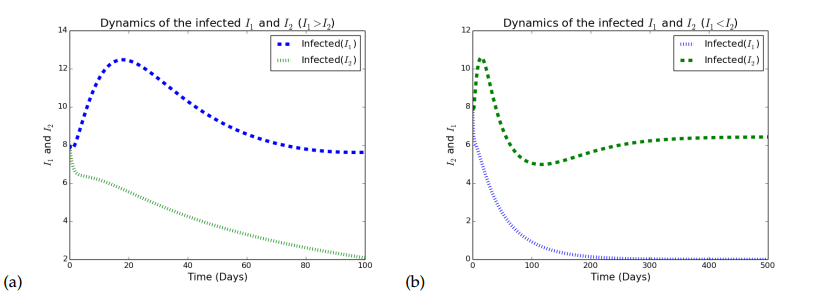
\begin{align*} \mathcal{F}_2 - \mathcal{V}_2 = \begin{pmatrix} \dfrac{\beta_2 \tilde{I_2} S}{N} \\[5pt] \dfrac{\beta_2\tilde{I_2} I_1}{N} \\[5pt] 0 \\[5pt] 0 \end{pmatrix} - \begin{pmatrix} \dfrac{\beta_1 I_2\tilde{I}_1}{N} + (q_2 + \mu)I_2 - r_2 T_2 \\[5pt] -\dfrac{\beta_1 \tilde{I}_1 I_2}{N} - r_{12}T_{12} + (q_{12}+\mu)I_{12}\\[5pt] -q_2I_2 + (r_2+\mu)T_2 \\[5pt] -q_{12}I_{12} + (r_{12}+\mu)T_{12} \end{pmatrix}. \end{align*} We then compute the Jacobian of the following \(F_2\) and \(V_2\) at strain \(2\) to obtain \begin{align*} F_2 & = \begin{pmatrix} \beta_2 S^{*} & \beta_2 S^{*} & 0 & 0 \\[5pt] \beta_2 I^{*}_{1} & \beta_2 I_1^{*} & 0 & 0 \\[5pt] 0 & 0 & 0 & 0 \\[5pt] 0 & 0 & 0 & 0 \end{pmatrix}\quad \text{and} \quad V_2 = \begin{pmatrix} \beta_1 I_1^{*} + q_2 + \mu & 0 & -r_2 & 0 \\[5pt] -\beta_1 I_{1}^{*} & (q_{12} + \mu) & 0 & -r_{12}\\[5pt] -q_2 & 0 & r_2+\mu & 0 \\[5pt] 0 & -q_{12} & 0 & r_{12}+\mu \end{pmatrix}. \end{align*} The dominant eigenvalue of the matrix which is determined by \(F_1V_1^{-1}\) and is the invasion reproductive number \(\tilde{R}_2\) is given by \begin{align*} \tilde{R}_2 = \frac{\beta_2}{\mu} \bigg[ \frac{\textbf{M} + \textbf{N} + {\left(\textbf{O} + \textbf{P} + {\left(\beta_{2} \mu^{2} + \beta_{2} \mu q_{12} + \beta_{2} \mu r_{12}\right)} r_{2}\right)} S}{\mu^{3} + \mu^{2} q_{12} + \textbf{Q} + {\left(\mu^{2} + \mu q_{12}\right)} q_{2} + {\left(\mu^{2} + \mu q_{2}\right)} r_{12} + {\left(\mu^{2} + \mu q_{12} + \mu r_{12}\right)} r_{2}} \bigg], \end{align*} where \begin{align*} \textbf{M} & = {\left(\beta_{1} \mu^{2} + \beta_{1}\mu r_{12} + {\left(\beta_{1}\mu + \beta_{1} r_{12}\right)} r_{2}\right)} I_{1}^{2}, \\[5pt] \textbf{N} &= {\left(\mu^{3} + \mu^{2} q_{2} + {\left(\mu^{2} +\mu q_{2}\right)} r_{12} + {\left(\mu^{2} + \mu r_{12}\right)} r_{2}\right)} I_{1}, \\[5pt] \textbf{O} & = \mu^{3} + \mu^{2} q_{12} + \mu^{2} r_{12}, \\[5pt] \textbf{P} & = {\left(\beta_{1} \mu^{2} + \beta_{1} \mu r_{12} + {\left(\beta_{1}\mu + \beta_{1}r_{12}\right)} r_{2}\right)} I_{1}, \\[5pt] \textbf{Q} & = {\left(\beta_{1} \mu^{2} + \beta_{1} \mu q_{12} + \beta_{1} \mu r_{12} + {\left(\beta_{1} \mu + \beta_{1} q_{12} + \beta_{1} r_{12}\right)} r_{2}\right)} I_{1}. \end{align*} After some algebraic manipulations, \(\tilde{R}_2\) can further be expressed as \begin{align*} \tilde{R}_2 = R_2\dfrac{\mu(a_1)}{\pi(\mu+r_2)}\dfrac{s^*\mu q_{12}(\mu+r_2\beta_2)+(\mu+r_{12})(\mu+r_2)i^{*^2}_1\beta_1+i^*_1(\mu q_2 +(\mu+r_2)(\mu+s^*\beta_1))+s^*\mu(\mu+r_2\beta_2))}{(\mu+q_{12}+r_{12})(\mu q_2+(\mu+r_2)(\mu+i^*\beta_1))} \end{align*} where \(a_1 = \mu+q_2+r_2\) and \(s^*, i^*_1\) is defined in \(E_1\). Similarly, \(\tilde{R}_2\) is essentially \(R_2\) multiplied by a term representing an altered vulnerability to infection with strain \(2\).

4. Numerical simulations

To support the analytical results, numerical simulations of the model system 1 are provided. Model parameter values used for the numerical simulations are listed in Table 1. For the purpose of illustration, we assumed heuristic model parameter values within realistic range for some of the model parameter values, and the following initial values: \(S = 30\), \(I_{1} = 8\), \(I_{2} = 8\), \(I_{12} = 8\) , \(T_{1} = 3\), \(T_{2} = 3\), \(T_{12} = 3\).

Figure 2 depicts the graphical representation of infectious individuals with HSV1 and HSV when either \(R_1>1>R_2\) Figure 2(a) or \(R_2>1>R_1\) Figure 2(b). In Figure 2(a), strain 1 dominates while in Figure 2(b), strain 2 dominates.

Figure 2. Simulations of model (1) showing plots with HSV strain 1 and HSV strain 2 as a function of time with various initial conditions(a)~ \(R_1>1>R_2\) ~(\(\beta_1=0.007\) , \(\beta_2=0.001\)), so that \(R_1=3.3684\),\(R_2=0.4812\) and \(R_0=3.3684\). ~(b)~\(R_2>1>R_1\)~ (\(\beta_1=0.001\), \(\beta_2=0.007\)), so that \(R_1=0.4812\), \(R_2=3.3684\) and \(R_0=3.3684\). Parameter values used are in Table 1.

Next, we illustrate the effects of increasing treatment rates on the dynamics of population with HSV1 and HSV2 in Figure 3.

Figure 3. Simulations of model (1) showing plots of individuals infected with HSV1~\(I_1\), as a function of time with respective to Treatment class \(T_1\) at different treatment rates at initial conditions \(S=30,~I_1=8,~I_2=8,~I_{12}=8,~T_1=3,~T_2=3,~T_{12}=3\). ~(a) Population with HSV1 and its respective treatment class at a lower treatment rate such that~\(q_1 = 0.45\),~\(q_2 = 0.45\),~\(q_{12} = 0.45\). ~(b) Population with HSV1 with treatment rate being increased to \(0.65\).~\(q_1 = 0.65\),~\(q_2 = 0.65\),~\(q_{12} = 0.65\). ~(c) Population with HSV1 with treatment rates being further increased to \(0.95\) such that~\(q_1 = 0.95\),~\(q_2 = 0.95\),~\(q_{12} = 0.95\).

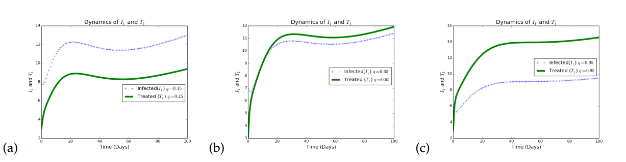
Figure 3 illustrates the effects of increasing treatment as a control strategy in a given population. In Figure 3(a), it is observed that when treatment rates with respect to HSV1 is small, the infected individuals increases. In Figure 3(b), the treatment rates for HSV1 infection is increased to a very reasonable value (\(0.65\)) and it is observed that although there is a reduction in the number of infected individuals, the impact is minimal. The treatment rate for the HSV1 is further increased to a reasonably high value (\(0.95\)) and it is observed that the infection persists, but at a lower rate. Thus, treatment only minimizes the rate of transmitting HSV strain 1, but does not eradicate it, which agrees with what is know about this disease that treatment is only palliative.

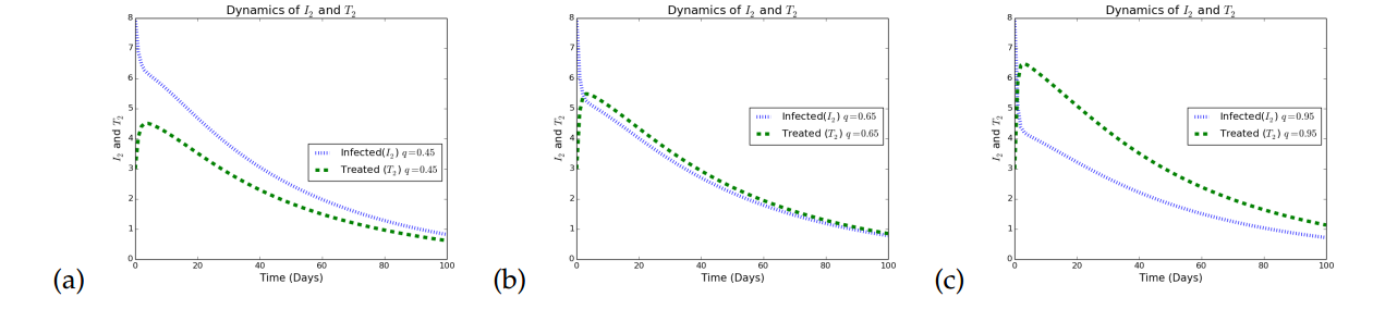
Simulations in Figure 4 illustrates the effects of increasing treatment as a control strategy in a given population. In Figure 4(a), it is observed that when treatment rates with respect to HSV2 is small, the infected individuals increases. In Figure 4(b) the treatment rate for HSV2 infection was increased to a very reasonable value (\(0.65\)) and it is observed that although there is a reduction in the number of infected individuals the impact is not that great. The treatment rate for the HSV2 was further increased to a reasonably high value (\(0.95\)) and it is observed that the infection persists but at a lower rate. Again, treatment only minimizes the rate of transmitting HSV strain 2, but does not eradicate it, which agrees with what is know about HSV that treatment only palliative.

Figure 4. Simulations of model (1) showing plots of individuals with HSV2~\(I_2\) as a function of time with its to Treatment class \(T_2\) and different treatment rates at initial conditions \(S=30,~I_1=8,~I_2=8,~I_{12}=8,~T_1=3,~T_2=3,~T_{12}=3\). ~(a) Population with HSV2 and its respective treatment class \(T_{12}\), at a lower treatment rate ~\(q_1 = 0.45\),~\(q_2 = 0.45\),~\(q_{12} = 0.45\). ~(b) Population with HSV2 and its respective treatments classes with treatment rate being increased to \(0.65\).~\(q_1 = 0.65\),~\(q_2 = 0.65\),~\(q_{12} = 0.65\). ~(c) Population with HSV2 and it respective treatment class with treatment being further increased to \(0.8\) such that~\(q_1 = 0.95\),~\(q_2 = 0.95\),~\(q_{12} = 0.95\). Parameter values used are in Table 1.

4.1. Sensitivity Analysis

Some of the model parameter values used herein were obtained from various sources, while the rest were assumed for illustrative purposes. Because errors could occur while collecting data or estimating model parameter values, it is important to investigate the sensitivity of the model parameters. In general, sensitivity analysis is to determine which model input parameters exert the most influence on the model results [33]. This information could then be used to tailor disease control strategy on the most sensitive parameters. Thus, we aim to investigate the relative importance of each parameter on the transmission dynamic of the disease, using the normalized forward sensitivity method [34]. This approach states that sensitivity indices are determined when a change in parameter allow us to measure the relative change in a state variable. It is important to note that while some sensitivity methods are mathematically elegant and comprehensive, their results in many cases are comparable to those obtained from simpler techniques [35].

Using sage programming language, we derive the following:

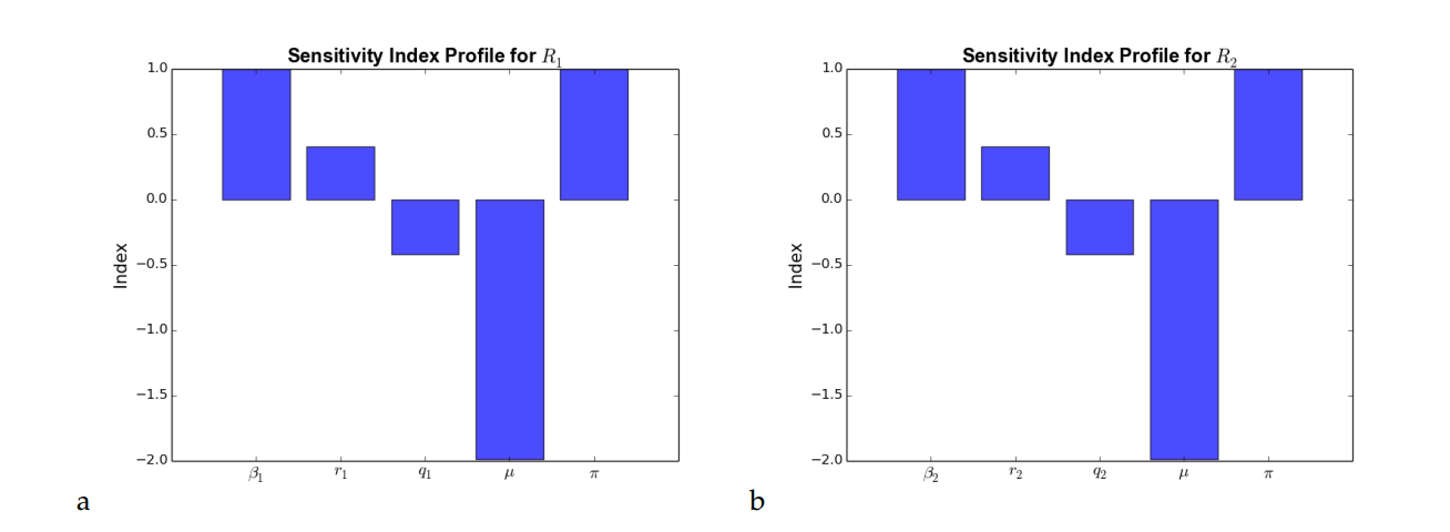
\begin{align*} \beta_1 &=\newcommand{\Bold}[1]{\mathbf{#1}}\frac{{\left(\mu \pi + \pi r_{1}\right)} \beta_{1}}{\beta_{1} \mu \pi + \beta_{1} \pi r_{1}},\\ r_1 &=\newcommand{\Bold}[1]{\mathbf{#1}}-\frac{{\left(\mu^{3} + \mu^{2} q_{1} + \mu^{2} r_{1}\right)} {\left(\frac{{\left(\beta_{1} \mu \pi + \beta_{1} \pi r_{1}\right)} \mu^{2}}{{\left(\mu^{3} + \mu^{2} q_{1} + \mu^{2} r_{1}\right)}^{2}} - \frac{\beta_{1} \pi}{\mu^{3} + \mu^{2} q_{1} + \mu^{2} r_{1}}\right)} r_{1}}{\beta_{1} \mu \pi + \beta_{1} \pi r_{1}},\\ q_1 &=\newcommand{\Bold}[1]{\mathbf{#1}}-\frac{\mu^{2} q_{1}}{\mu^{3} + \mu^{2} q_{1} + \mu^{2} r_{1}},\\ \\ \mu &=\newcommand{\Bold}[1]{\mathbf{#1}}\frac{\mu{\left(\mu^{3} + \mu^{2} q_{1} + \mu^{2} r_{1}\right)} {\left(\frac{\beta_{1} \pi}{\mu^{3} + \mu^{2} q_{1} + \mu^{2} r_{1}} - \frac{{\left(\beta_{1} \mu \pi + \beta_{1} \pi r_{1}\right)} {\left(3 \, \mu^{2} + 2 \, \mu q_{1} + 2 \, \mu r_{1}\right)}}{{\left(\mu^{3} + \mu^{2} q_{1} + \mu^{2} r_{1}\right)}^{2}}\right)}}{\beta_{1} \mu \pi + \beta_{1} \pi r_{1}},\\ \pi &=\newcommand{\Bold}[1]{\mathbf{#1}}\frac{{\left(\beta_{1} \mu + \beta_{1} r_{1}\right)} \pi}{\beta_{1} \mu \pi + \beta_{1} \pi r_{1}},\\ \beta_2 &=\newcommand{\Bold}[1]{\mathbf{#1}}\frac{{\left(\mu \pi + \pi r_{2}\right)} \beta_{2}}{\beta_{2} \mu \pi + \beta_{2} \pi r_{2}},\\ r_2 &=\newcommand{\Bold}[1]{\mathbf{#1}}-\frac{{\left(\mu^{3} + \mu^{2} q_{2} + \mu^{2} r_{2}\right)} {\left(\frac{{\left(\beta_{2} \mu \pi + \beta_{2} \pi r_{2}\right)} \mu^{2}}{{\left(\mu^{3} + \mu^{2} q_{2} + \mu^{2} r_{2}\right)}^{2}} - \frac{\beta_{2} \pi}{\mu^{3} + \mu^{2} q_{2} + \mu^{2} r_{2}}\right)} r_{2}}{\beta_{2} \mu \pi + \beta_{2} \pi r_{2}},\\ q_2 &=\newcommand{\Bold}[1]{\mathbf{#1}}-\frac{\mu^{2} q_{2}}{\mu^{3} + \mu^{2} q_{2} + \mu^{2} r_{2}}. \end{align*} Then, using the parameter values \(\beta_1 = 0.007\), \(\beta_2 = 0.001\), \(r_1= 0.6\), \(r_2= 0.6\), \(q_1 = 0.45\), \(q_1 = 0.45\), \(\mu = 0.019\), \(\pi = 0.3\), we compute the sensitivity indices of \(R_1\) and \(R_2\) which are summarized in Tables 2 and 3.
Table 2. Sensitivity indices of \(R_1\).
Parameter Sensitivity index
\(\beta_1\) \(1.00000\)
\(r_1\) \(0.408033 \)
\(q_1\) \(-0.42095\)
\(\mu \) \(-1.98708\)
\(\pi \) \(1.00000\)
Table 3. Sensitivity indices of \(R_2\).
Parameter Sensitivity index
\(\beta_2\) \(1.00000\)
\(r_2\) \(0.408033 \)
\(q_2\) \(-0.42095\)
\(\mu \) \(-1.98708\)
\(\pi \) \(1.00000\)

From Tables 2 and 3, the sensitivity index with positive sign indicate that the value of the reproduction numbers \(R_1\) and \(R_2\) increase when the corresponding parameters increase while the parameters with negative signs indicate that, for an increase in the corresponding parameters, there is a decrease in the value of the reproduction numbers \(R_1\) and \(R_2\). Using the model parameter values in Table 1, we graphically represent the sensitivity index profile of the reproduction numbers \(R_1\) and \(R_2\).

From Figure 5(a) and Figure 5(b), it can be observed that \(\beta_1\), \(\beta_2\) and \(\pi\) have the highest influence on the reproduction number \(R_0\) followed by \(\mu\), \(q_1\) and \(q_2\). This implies that an increase in the contact rates \(\beta_1\), \(\beta_2\) and recruitment/inflow rate \(\pi\) will lead to a corresponding increase in the basic reproduction number. On the other hand, \(\mu\), \(q_2\) and \(q_1\) correlates negatively with the basic reproduction number as an increase in such parameters will lead to a corresponding decrease in the basic reproduction number.

Figure 5. a) Effect of the various parameters (\(\beta_ 1\) , \(r_ 1\) , \(q_ 1\) , \(\mu\) and \(\pi\)) which correspond to \(R_1\) on the reproduction number \(R_0\). b) Effect of the various parameters (\(\beta_ 2\) , \(r_ 2\) , \(q_ 2\) , \(\mu\) and \(\pi\)) which correspond to \(R_2\) on the reproduction number \(R_0\).

5. Conclusion

We formulated and analyzed a mathematical model for the transmission of HSV infection with palliative treatment. Individuals from the susceptible compartments could either be infected with strain 1 or strain 2 of the disease. Infected individuals could then either go for treatment or get infected with the other strain (co-infection) and also receive treatment. Since this disease has no cure, the treatment only reduces the intensity of the disease but does not cure it. The model is then analyzed qualitatively with numerical simulations provided to support the theoretical results. The model basic reproduction number is computed for both strains independently with \(R_0=max \lbrace R_1, R_2 \rbrace \), and used to investigate the stability of the model equilibria. The disease-free equilibrium of the proposed model is locally-asymptotically stable when the basic reproduction number \(R_0=max\lbrace R_1, R_2 \rbrace \) is less than unity. Numerical simulations indicate that the two HSV strains co-exist, with HSV1 dominating but not driving out HSV2 whenever \(R_1 > R_2 > 1\) and vice versa. If infection with one strain confers incomplete immunity against the other, the model 1 exhibits the phenomenon of competitive exclusion, where the first strain HSV1 could drive out the second strain HSV2 when \(R_1 > 1 > R_2\). Using the method in [32], we establish existence and local stability of single strain equilibria through invasion reproductive numbers. In order to determine the relative importance of model parameters to initial disease transmission, sensitivity analysis is carried out. The reproduction number is most sensitive respectively to the contact rates \(\beta_1\) and \(\beta_2\) as well as the recruitment rate \( \pi \). The application of control measures such as palliative treatment has an impact on the infection dynamics, but does not completely eradicate the disease. This study is not exhaustive as there are a number of limitations. Treatment could significantly help to minimize transmission of the disease but not eradicate it (because it is only a palliative measure), development of treatment resistance is to be expected [36]. Also, while there is no definitive vaccine, studies have shown that even an imperfect prophylactic HSV-2 vaccine could have an important public health benefits on HSV-2 incidence [14]. Future studies accounting for heterogeneity in infection rates such as by age, sex and sexual activity and incorporating the above limitations are viable.

Acknowledgments

JK thanks the African Institute for Mathematical Science (AIMS-Tanzania) for financial support towards her M.Sc. in mathematical sciences.

Author Contributions

All authors contributed equally to the writing of this paper. All authors read and approved the final manuscript.

Conflicts of Interest

''The authors declare no conflict of interest.''

References

  1. Smith, J. S., & Robinson, N. J. (2002). Age-specific prevalence of infection with herpes simplex virus types 2 and 1: a global review. The Journal of Infectious Diseases, 186(Supplement1), S3-S28. [Google Scholor]
  2. Stevens, J. G. (1975). Latent herpes simplex virus and the nervous system. Current Topics in Microbiology and Immunology, 31-50. [Google Scholor]
  3. Looker, K. J., Magaret, A. S., Turner, K. M. E., Vickerman, P., Gottlieb, S. L., & Newman, L. M. (2015). Global estimates of prevalent and incident herpes simplex virus type 2 infections in 2012. PloS ONE, 10(1), e114989. https://doi.org/10.1371/journal.pone.0114989. [Google Scholor]
  4. Fisman, D. N., Lipsitch, M., Hook III, E. W., & Goldie, S. J. (2002). Projection of the future dimensions and costs of the genital herpes simplex type 2 epidemic in the united states. Sexually Transmitted Diseases, 29(10), 608-622. [Google Scholor]
  5. Hill, T. J. (1985). Herpes simplex virus latency. In The herpesviruses (pp. 175-240). Springer, Boston, MA. [Google Scholor]
  6. Paine Jr, T. F. (1964). Latent herpes simplex infection in man. Bacteriological Reviews, 28(4), 472-479. [Google Scholor]
  7. Whitley, R. J., Kimberlin, D. W., & Roizman, B. (1998). Herpes simplex viruses. Clinical Infectious Diseases, 541-553. [Google Scholor]
  8. Blower, S., & Ma, L. (2004). Calculating the contribution of herpes simplex virus type 2 epidemics to increasing HIV incidence: treatment implications. Clinical Infectious Diseases, 39(Supplement_5), S240-S247. [Google Scholor]
  9. Schiffer, J. T., Swan, D. A., Magaret, A., Schacker, T. W., Wald, A., & Corey, L. (2016). Mathematical modeling predicts that increased HSV-2 shedding in HIV-1 infected persons is due to poor immunologic control in ganglia and genital mucosa. PloS one, 11(6), e0155124. https://doi.org/10.1371/journal.pone.0155124. [Google Scholor]
  10. Freeman, E. E., Weiss, H. A., Glynn, J. R., Cross, P. L., Whitworth, J. A., & Hayes, R. J. (2006). Herpes simplex virus 2 infection increases HIV acquisition in men and women: systematic review and meta-analysis of longitudinal studies. Aids, 20(1), 73-83. [Google Scholor]
  11. Forward, K. R., & Lee, S. H. (2003). Predeominace of herpes simplex virus type 1 from patients with genital herpes in nova scotia. Canadian Journal of Infectious Diseases, 14(2), 94-96. [Google Scholor]
  12. Ryan, K. J., & Ray, C. G. (2004). Medical Microbiology. McGraw Hill, 4, 370. [Google Scholor]
  13. Straface, G., Selmin, A., Zanardo, V., De Santis, M., Ercoli, A., & Scambia, G. (2012). Herpes simplex virus infection in pregnancy. Infectious Diseases in Obstetrics and Gynecology, 2012, Article ID 385697, https://doi.org/10.1155/2012/385697. [Google Scholor]
  14. Spicknall, I. H., Looker, K. J., Gottlieb, S. L., Chesson, H. W., Schiffer, J. T., Elmes, J., & Boily, M. C. (2019). Review of mathematical models of HSV-2 vaccination: Implications for vaccine development. Vaccine, 37(50), 7396-7407. [Google Scholor]
  15. Corey, L., Adams, H. G., Brown, Z. A., & Holmes, K. K. (1983). Genital herpes simplex virus infections: clinical manifestations, course, and complications. Annals of Internal Medicine, 98(6), 958-972. [Google Scholor]
  16. ACOG Practice Bulletin 57 (2004). Gynecologic Herpes Simplex Virus Infections. Obstetrics & Gynecology, 104(5), 1111-1118. [Google Scholor]
  17. Corey, L., Wald, A., Patel, R., Sacks, S. L., Tyring, S. K., Warren, T., ... & Vargas-Cortes, M. (2004). Once-daily valacyclovir to reduce the risk of transmission of genital herpes. New England Journal of Medicine, 350(1), 11-20. [Google Scholor]
  18. Gupta, R., Wald, A., Krantz, E., Selke, S., Warren, T., Vargas-Cortes, M., ... & Corey, L. (2004). Valacyclovir and acyclovir for suppression of shedding of herpes simplex virus in the genital tract. The Journal of Infectious Diseases, 190(8), 1374-1381. [Google Scholor]
  19. Mok, W., Stylianopoulos, T., Boucher, Y., & Jain, R. K. (2009). Mathematical modeling of herpes simplex virus distribution in solid tumors: implications for cancer gene therapy. Clinical Cancer Research, 15(7), 2352-2360. [Google Scholor]
  20. Chamchod, F., & Britton, N. F. (2012). On the dynamics of a two-strain influenza model with isolation. Mathematical Modelling of Natural Phenomena, 7(3), 49-61. [Google Scholor]
  21. Esteva, L., & Vargas, C. (2003). Coexistence of different serotypes of dengue virus. Journal of Mathematical Biology, 46(1), 31-47. [Google Scholor]
  22. Li, X. Z., Liu, J. X., & Martcheva, M. (2010). An age-structured two-strain epidemic model with super-infection. Mathematical Biosciences & Engineering, 7(1), 123. [Google Scholor]
  23. Sharomi, O., & Gumel, A. B. (2008). Dynamical analysis of a multi-strain model of HIV in the presence of anti-retroviral drugs. Journal of Biological Dynamics, 2(3), 323-345. [Google Scholor]
  24. Nuno, M., Feng, Z., Martcheva, M., & Castillo-Chavez, C. (2005). Dynamics of two-strain influenza with isolation and partial cross-immunity. SIAM Journal on Applied Mathematics, 65(3), 964-982. [Google Scholor]
  25. Schiffer, J. T., Swan, D. A., Magaret, A., Corey, L., Wald, A., Ossig, J., ... & Birkmann, A. (2016). Mathematical modeling of herpes simplex virus-2 suppression with pritelivir predicts trial outcomes. Science Translational Medicine, 8(324), 324ra15-324ra15. [Google Scholor]
  26. Bryson, Y., Dillon, M., Bernstein, D. I., Radolf, J., Zakowski, P., & Garratty, E. (1993). Risk of acquisition of genital herpes simplex virus type 2 in sex partners of persons with genital herpes: a prospective couple study. Journal of Infectious Diseases, 167(4), 942-946. [Google Scholor]
  27. Bhunu, C. P., Mhlanga, A. N., & Mushayabasa, S. (2014). Exploring the impact of prostitution on HIV/AIDS transmission. International Scholarly Research Notices, 2014, Article ID 651025, https://doi.org/10.1155/2014/651025. [Google Scholor]
  28. Podder, C. N., & Gumel, A. B. (2010). Qualitative dynamics of a vaccination model for HSV-2. IMA Journal of Applied Mathematics, 75(1), 75-107. [Google Scholor]
  29. van den Driessche, P., & Watmough, J. (2002). Reproduction numbers and subthreshold endemic equilibria for compartmental models of disease transmission. Mathematical Biosciences 180(1-2), 29-48. [Google Scholor]
  30. Thowsen, A. (1981). The Routh-Hurwitz method for stability determination of linear differential-difference systems. International Journal of Control, 33(5), 991-995. [Google Scholor]
  31. Castillo-Chavez, C., Feng, Z., & Huang, W. (2002). On the computation of \(R_0\) and its role in global stability. IMA Volumes in Mathematics and Its Applications, 125, 229-250. [Google Scholor]
  32. Crawford, B., & Kribs-Zaleta, C. M. (2009). The impact of vaccination and coinfection on HPV and cervical cancer. Discrete & Continuous Dynamical Systems-B, 12(2), 279-304. [Google Scholor]
  33. Samsuzzoha, M., Singh, M., & Lucy, D. (2013). Uncertainty and sensitivity analysis of the basic reproduction number of a vaccinated epidemic model of influenza. Applied Mathematical Modelling 37, 903-915. [Google Scholor]
  34. Chitnis, N., Hyman, J. M., & Cushing, J. M. (2008). Determining important parameters in the spread of malaria through the sensitivity analysis of a mathematical model. Bulletin of Mathematical Biology, 70(5), 1272-1296. [Google Scholor]
  35. Hamby, D. (1995). A comparison of sensitivity analysis techniques. Health Physics 68(2), 195-204. [Google Scholor]
  36. Lipsitch, M., Bacon, T. H., Leary, J. J., Antia, R., & Levin, B. R. (2000). Effects of antiviral usage on transmission dynamics of herpes simplex virus type 1 and on antiviral resistance: Predictions of mathematical models. Antimicrobial Agents and Chemotherapy, 44(10), 2824-2835. [Google Scholor]