Convergence analysis for a new faster four steps iterative algorithm with an application

1. Introduction

Throughout this paper, let \(\Gamma\) be a nonempty closed subset of a real Banach space \(\Psi\), \(\mathbb{N}\) the set of all natural numbers, \(\Re\) the set of all real numbers and \(C([d,e])\) denotes the set of all continuous real-valued functions defined on \([d,e]\subset\Re\).

A mapping \(T:\Gamma\to \Gamma\) is called

• \(\bullet\) contraction if there exists a constant \(\delta\in[0,1)\) such that
  \begin{eqnarray} \|T\psi-T\zeta\|\leq \delta\|\psi-\zeta\|,\,\,\forall\,\psi,\zeta\in \Gamma; \end{eqnarray}

  (1)
• \(\bullet\) nonexpansive if
  \begin{eqnarray} \|T\psi-T\zeta\|\leq \|\psi-\zeta\|,\,\,\forall\,\psi,\zeta\in \Gamma. \end{eqnarray}

  (2)

Clearly, every contraction map is a nonexpansive map for \(\delta=1\).

For some decades now, fixed point theory has been developed into a basic and an essential tool for different branches of both applied and pure mathematics. Particularly, it may be seen as an essential subject of nonlinear functional analysis. Moreover, fixed point theory is one of the useful tools to solve many problems in applied sciences and engineering such as: the existence of solutions to integral equations, differential equations, matrix equations, dynamical system, models in economy, game theory, fractals, graph theory, optimization theory, approximation theory, computer science and many other subjects.

It is well known that several mathematical problems are naturally formulated as fixed point problem,

where \(T\) is some suitable mapping, which may be nonlinear. For example, given a mapping \(\varphi:[d,e]\subset\Re\to \Re\) and \(k:[d,e]\times[d,e]\times\Re\to \Re\), then the solution to the following nonlinear integral equation: where \(\psi\in C([d,e])\), is tantamount to finding the fixed point of the integral operator \(T:C([d,e])\to C([d,e])\) defined by for all \(\psi \in C([d,e])\).

A solution \(\psi\) of the problem (3) is called a fixed point of the mapping \(T\). We will denote the set of all fixed points of \(T\) by \(F(T)\), i.e., \(F(T)=\{\psi\in \Gamma: T\psi=\psi\}\).

On the other hand, once the existence of some fixed points of a given mapping is guaranteed, then finding such fixed point of the mapping is cumbersome in some cases. To surmount this difficulty, iterative algorithm is usually employed for approximating them. An efficient iterative should at least be \(T\)-stable, converges faster than a number of some existing iterative scheme in the literature, converges to a fixed point of an operator or should be data dependent (see [1]).

The Picard iterative algorithm

is one of the first iterative algorithms which has been widely used for approximating the fixed points of contraction mappings. However, the success of Picard iterative algorithm has not been carried over to the more general classes of operators such as nonexpansive mappings even when a fixed exists.

For example, the mapping \(T:[0,1]\to[0,1]\) defined by \(T\psi=1-\psi\) for all \(\psi\in [0,1]\) is a nonexpansive mapping with a unique fixed point \(\psi=\frac{1}{2}\). Notice that for \(\psi_0\in [0,1]\), \(\psi_0\neq\frac{1}{2}\), the Picard iterative algorithm (6) generates the sequence \(\{1-\psi_0,\psi_0,1-\psi_0,...\}\) for which fails to converge to the fixed point \(z\) of \(T\).

To overcome the failure recorded by Picard iterative algorithm, many researchers in nonlinear analysis got busy with constructing several new iterative algorithms for approximating the fixed points of nonexpansive mappings and other mappings more general than the classes of nonexpansive mappings.

Some notable iterative algorithms in the existing literature includes: Mann [2], Ishikawa [3], Noor [4], Argawal et al., [5], Abbas and Nazir [6], SP [7], S* [8], CR [9], Normal-S [10], Picard-S [11], Thakur et al., [12], M [13], M* [14], Garodia and Uddin [15], Two-Step Mann [16] iterative algorithms and so on.

In 2007, the following iterative algorithm which is known as S iteration was introduced by Argawal et al., [5]:

where \(\{\mu_s\}\) and \(\{r_s\}\) are sequences in \([0,1].\)

In 2014, the following iterative algorithm known as Picard-S iteration was introduced by Gursoy and Karakaya [11]:

where \(\{\mu_s\}\) and \(\{r_s\}\) are sequences in \([0,1].\) The authors showed with the aid of an example that Picard-S iterative algorithm (8) converges at a rate faster than all of Picard, Mann, Ishikawa, Noor, SP, CR, S, S*, Abbas and Nazir, Normal-S and Two-Step Mann iteration processes for contraction mappings.

In 2016, Thakur et al., [12] introduced the following three steps iterative algorithm:

where \(\{\mu_s\}\) and \(\{r_s\}\) are sequences in \([0,1].\) With the help of numerical example, they proved that (9) is faster than Picard, Mann, Ishikawa, Agarwal, Noor and Abbas iterative algorithm for Suzuki generalized nonexpansive mappings.

In 2018, Ullah and Arshad [13] introduced the M iterative algorithm as follows:

where \(\{r_s\}\) is a sequence in \([0,1].\) Numerically they show that M iterative algorithm (10) converges faster than S iterative algorithm (7) and Picard-S iteration process (8) for Suzuki generalized nonexpansive mapping.

Recently, Garodia and Uddin [15] introduced the following three steps iterative algorithm:

where \(\{r_s\}\) is a sequence in \([0,1].\) The authors showed both analytically and numerically that their iterative algorithm (11) converges faster than M iterative algorithm (10). Also, they showed that the iterative algorithm (11) converges faster than all of S, Abbas and Nazir, Thakur New, M, Noor, Picard-S, Thakur, M* iterative algorithms for contractive-like mappings and Suzuki generalized nonexpansive mappings.

Clearly, from the performance of the iterative algorithm (11), we note that it is one of the leading iterative schemes.

Problem 1. Is it possible to construct a four-steps iterative algorithm which have better rate of converges than the three-step iterative algorithm (11) for contraction mappings?

To solve the above problem, we introduce the following iterative algorithm, called AU iterative algorithm: where \(\{r_s\}\) is a sequence in \([0,1]\).

The aim of this paper is to prove the strong convergence of AU iterative algorithm (12) to the fixed points of contraction mappings. We will prove analytically that AU iterative algorithm (12) converges faster than the iterative algorithm (11). With the aid of an example, we show numerically that AU iterative algorithm has a better rate of convergence than the iterative algorithm (11) and several other leading iterative algorithms existing in the literature. Also, we will show that AU iterative algorithm is \(T\)-stable and data dependent.

Additionally, we will use AU iterative algorithm (12) to find the unique solutions of a nonlinear integral equation.

2. Preliminaries

The following definitions and lemmas will be useful in proving our main results.

Definition 2.[17] Let \(\{a_s\}\) and \(\{b_s\}\) be two sequences of real numbers that converge to \(a\) and \(b\) respectively and assume that there exists \begin{eqnarray*} \ell=\lim\limits_{s\to\infty}\frac{\|a_s-a\|}{\|b_s-b\|}. \end{eqnarray*}Then,

• (\(R_1\)) if \(\ell=0\), we say that \(\{a_s\}\) converges faster to \(a\) than \(\{b_s\}\) does to \(b\).
• (\(R_2\)) If \(0< \ell< \infty\), we say that \(\{a_s\}\) and \(\{b_s\}\) have the same rate of convergence.

Definition 3. [17] Let \(\{\omega_s\}\) and \(\{\mu_s\}\) be two fixed point iteration processes that converge to the same point \(z\), the error estimates \begin{eqnarray*} \|\omega_s-z\|&\leq& a_s, \,\,s \in\mathbb{N},\\ \|\mu_s-z\|&\leq& b_s, \,\,s \in\mathbb{N}, \end{eqnarray*}are available where \(\{a_s\}\) and \(\{b_s\}\) are two sequences of positive numbers converging to zero. Then we say that \(\{\omega_s\}\) converges faster to \(z\) than \(\{\mu_s\}\) does if \(\{a_s\}\) converges faster than \(\{b_s\}\).

Definition 4.[17] Let \(T\), \(\tilde{T}:\Gamma\to \Gamma\) be two operators. We say that \(\tilde{T}\) is an approximate operator for \(T\) if for some \(\epsilon>0\), we have

Definition 5.[18] Let \(\{\zeta_s\}\) be any sequence in \(\Gamma\). Then, an iterative algorithm \(\psi_{s+1}=f(T,\psi_s)\), which converges to fixed point \(z\), is said to be \(T\)-stable if for \(\varepsilon_s=\|\zeta_{s+1}-f(T,\zeta_s)\|\), \(\forall\,s\in\mathbb{N}\), we have

Lemma 6. [19] Let \(\{ \mathfrak{\theta}_s\}\) and \(\{\lambda_s\}\) be nonnegative real sequences satisfying the following inequalities:

where \(\sigma_s\in (0,1)\) for all \(s\in \mathbb{N}\), \(\sum\limits_{s=0}^{\infty}\sigma_s=\infty\) and \(\lim\limits_{s\to\infty}\frac{ \mathfrak{\lambda}_s}{\sigma_s}=0\), then \(\lim\limits_{s\to\infty} \mathfrak{\theta}_s=0\).

Lemma 7. [20] Let \(\{ \mathfrak{\theta}_s\}\) be a nonnegative real sequence and there exits an \(s_0\in \mathbb{N}\) such that for all \(s\geq s_0\) satisfying the following condition: \begin{eqnarray*} \mathfrak{\theta}_{s+1}\leq(1-\sigma_s) \mathfrak{\theta}_s+\sigma_s \lambda_s, \end{eqnarray*}where \(\sigma_s\in (0,1)\) for all \(s\in \mathbb{N}\), \(\sum\limits_{s=0}^{\infty}\sigma_s=\infty\) and \(\lambda_s\geq0\) for all \(s\in \mathbb{N}\), then \begin{eqnarray*} 0\leq\limsup\limits_{s\to\infty} \mathfrak{\theta}_s\leq\limsup\limits_{s\to\infty}\lambda_s. \end{eqnarray*}

3. Convergence result

In this section, we prove the strong convergence of AU iterative algorithm (12) for contraction mappings.

Theorem 8. Let \(\Gamma\) be a nonempty closed convex subset of a real Banach space \(\Psi\) and \(T:\Gamma\to \Gamma\) be a contraction mapping such that \(F(T)\neq\emptyset\). Let \(\{\psi_s\}\) be the sequence iteratively generated by (12) with a real sequence \(\{r_s\}\) in \([0,1]\) satisfying \(\sum\limits_{s=0}^{\infty}r_s=\infty\). Then \(\{\psi_s\}\) converges strongly to a unique fixed point of \(T\).

Proof. Given \(z\in F(T)\), then from (12) we have

Now, from (12) and (16) we obtain Also, from (12) and (17) we get Finally, from (12) and (18) we have From (19), the following inequality is obtained: From (20), we have Since for all \(s\in \mathbb{N}\), \(\{r_s\}\in [0,1]\) and \(\delta\in (0,1)\), it follows that \((1-(1-\delta)r_s)< 1\). From classical analysis we know that \(1-\psi< \exp^{-\psi}\) for all \(\psi\in [0,1]\). Then from (21), we have If we take the limits of both sides of (22), we get \(\lim\limits_{s\to\infty}\|\psi_s-z\|=0\). Hence, \(\{\psi_s\}\) converges strongly to the fixed point of \(T\) as required.

4. Stability result

Theorem 9. Let \(\Gamma\) be a nonempty closed convex subset of a Banach space \(\Psi\) and \(T:\Gamma \to \Gamma\) be a contraction mapping. Let \(\{\psi_s\}\) be an iterative algorithm defined by (12) with a real sequence \(\{r_s\}\) in [0,1] satisfying \(\sum\limits_{s=0}^{\infty}r_s=\infty\). Then the iterative algorithm (12) is \(T\)-stable.

Proof. Let \(\{\zeta_s\}\subset \Psi\) be an arbitrary sequence in \(\Gamma\) and suppose that the sequence iteratively generated by (12) is \(\psi_{s+1}=f(T,\psi_s)\), which converges to a unique point \(z\) and that \(\varepsilon_s=\|\zeta_{s+1}-f(T,\zeta_s)\|\). To prove that (12) is T-stable, we have to show that \(\lim\limits_{s\to\infty}\varepsilon_s=0\Leftrightarrow \lim\limits_{s\to\infty}\zeta_s=z\).

Let \(\lim\limits_{s\to\infty}\varepsilon_s=0\). Then from (12) and the demonstration above, we have

Putting (24) into (23) we obtain Substituting (26) into (25), we obtain Substituting (28) into (27), we get For all \(s\in \mathbb{N}\), put \begin{eqnarray*} \theta_s&=&\|\zeta_s-z\|,\\ \sigma_s&=&(1-\delta)r_s\in (0,1),\\ \lambda_s&=&\varepsilon_s. \end{eqnarray*}Since \(\lim\limits_{s\to\infty}\varepsilon_s=0\), this implies that \(\frac{\lambda_s}{\sigma_s}=\frac{\varepsilon_s}{(1-\delta)r_s}\to 0\) as \(s\to\infty\). Apparently, all the conditions of Lemma 6 are fulfilled. Hence, we have \(\lim\limits_{s\to\infty}\zeta_s=z\).

Conversely, let \(\lim\limits_{s\to\infty}\zeta_s=z\). The we have

From (30), it follows that \(\lim\limits_{s\to\infty}\varepsilon_s=0\). Hence, our new iterative algorithm (12) is stable with respect to \(T\).

5. Rate of convergence

In this section, we show that AU iterative algorithm (12) converges faster than Garodia and Uddin iterative algorithm (11) for contraction mappings.

Theorem 10. Let \(\Gamma\) be a nonempty closed convex subset of a Banach space and \(T:\Gamma\to\Gamma\) be a contraction mapping with fixed point \(z\). For any \(w_0=\psi_0\in\Gamma\), let \(\{w_s\}\) and \(\{\psi_s\}\) be two sequences iteratively generated by (11) and (12) respectively, with real sequence \(\{r_s\}\in [0,1]\) such that \(r\leq r_s< 1\), for some \(r>0\) and \(s\in \mathbb{N}\). Then \(\{\psi_s\}\) converges faster to \(z\) than \(\{w_s\}\) does.

Proof. Recalling the inequality (21), we have

Following our assumption that \(r\leq r_s< 1\), for some \(r>0\) and together with \(s\in \mathbb{N}\), then from (31) we obtain Let Similarly, for any \(z\in F(T)\), it follows from (11) that Using (11) and (34), we obtain Again, from (11) and (35) we get From (36), we obtain the following inequalities: From (37), we have Then from (38) we obtain that Put Now, from (33) and (40) we have that Since \(\lim\limits_{s\to\infty}\frac{\theta_{s+1}}{\theta_{s}}=\lim\limits_{s\to\infty}\frac{\delta^{s+2}}{\delta^{s+1}}=\delta< 1\), so from ratio test we know that \(\sum\limits_{s=0}^{\infty}\theta_s< \infty\). Hence, from (41) we have From the above demonstrations, it implies that \(\{\psi_s\}\) converges at a rate faster than \(\{w_s\}\). Hence, our new iterative algorithm (12) converges faster than Garodia and Uddin iterative algorithm (11). To support the analytical proof of Theorem 10 and to illustrate the efficiency of AU iterative algorithm (12), we will consider the following numerical example.

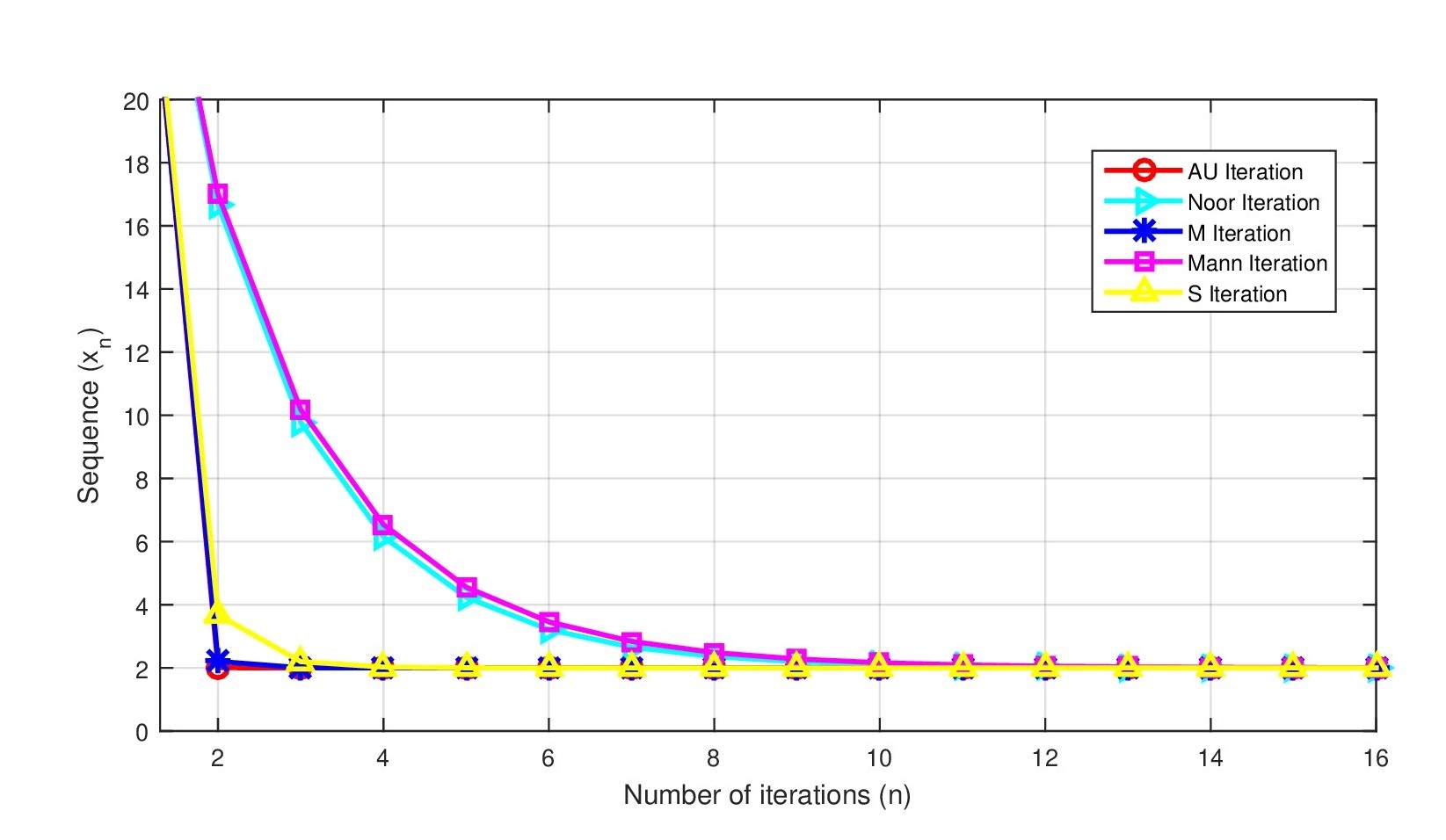
Example 1. Let \(\Psi=\Re\) and \(\Gamma=[1,50]\). Let \(T:\Gamma\to\Gamma\) be a mapping defined by \(T\psi=\sqrt[3]{2\psi+4}\) for all \(\psi\in \Gamma\). Clearly, \(T\) is contraction and \(z=2\) is a fixed point of \(T\). Take \(\mu_s=r_s=\frac{1}{2}\), with an initial value of 30.

By using the above example, we will show that AU iterative algorithm (12) converges faster a number of leading iterative algorithms in existing literature.

Table 1.A comparison of the different iterative algorithm.

Step	S	MANN	M	NOOR	AU
1	30.000000000	30.000000000	30.000000000	30.000000000	30.000000000
2	3.6809877034	17.000000000	2.2052183845	16.671526557	2.0055900713
3	2.1987214827	10.180987703	2.0032795388	9.7690754673	2.0000025151
4	2.0258396187	6.5399580891	2.0000531287	6.1528499922	2.0000000011
5	2.0034028155	4.5576312697	2.0000008609	4.2363659316	2.0000000000
6	2.0004488682	3.4579473856	2.0000000139	3.2106233814	2.0000000000
7	2.0000592237	2.8381224183	2.0000000002	2.6575629271	2.0000000000
8	2.0000078142	2.4845256350	2.0000000000	2.3578892859	2.0000000000
9	2.0000010310	2.2811112127	2.0000000000	2.1950165817	2.0000000000
10	2.0000001360	2.1634532374	2.0000000000	2.1063366837	2.0000000000
11	2.0000000179	2.0951662880	2.0000000000	2.0580036416	2.0000000000
12	2.0000000024	2.0554515931	2.0000000000	2.0316457914	2.0000000000
13	2.0000000003	2.0323255723	2.0000000000	2.0172673331	2.0000000000
14	2.0000000000	2.0188493597	2.0000000000	2.0094223922	2.0000000000
15	2.0000000000	2.0109929989	2.0000000000	2.0051417581	2.0000000000
16	2.0000000000	2.0064117448	2.0000000000	2.0028058861	2.0000000000

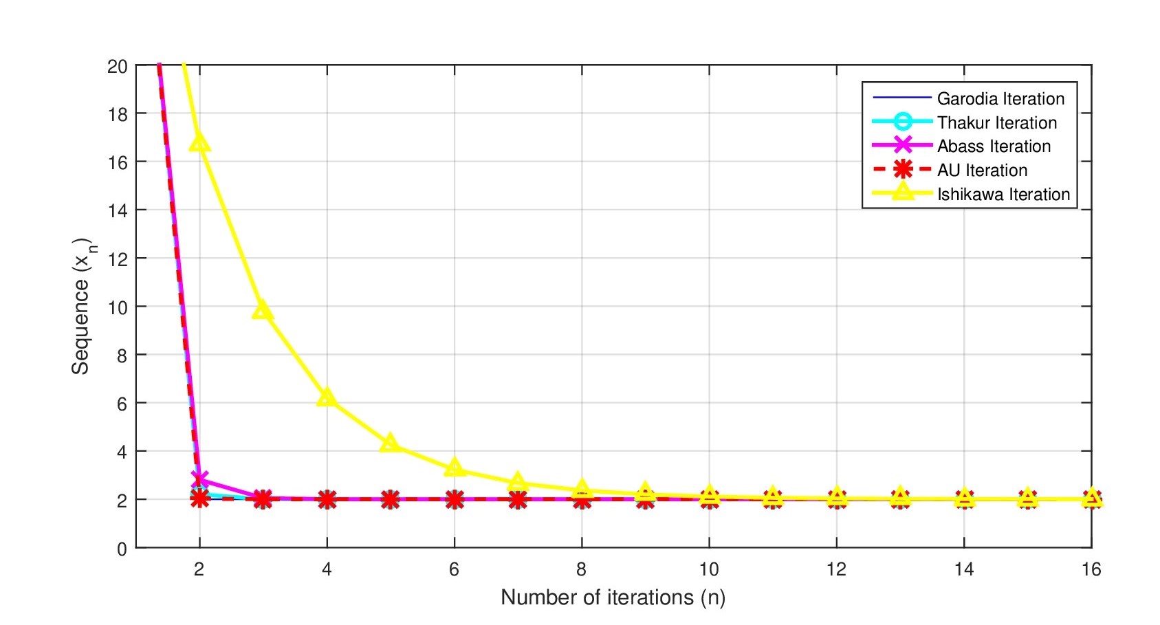
Table 2. A comparison of the different Iterative methods.

Step	ISHIKAWA	GARODIA	ABBASS	THAKUR	AU
1	30.000000000	30.000000000	30.000000000	30.000000000	30.000000000
2	16.680987703	2.0287550076	2.8050437150	2.2052183845	2.0055900713
3	9.7832248288	2.0000774455	2.0456798729	2.0032795388	2.0000025151
4	6.1683753023	2.0000002091	2.0027147499	2.0000531287	2.0000000011
5	4.2509176634	2.0000000006	2.0001617881	2.0000008609	2.0000000000
6	3.2228294683	2.0000000000	2.0000096435	2.0000000139	2.0000000000
7	2.6669712534	2.0000000000	2.0000005748	2.0000000002	2.0000000000
8	2.3646881630	2.0000000000	2.0000000343	2.0000000000	2.0000000000
9	2.1996958627	2.0000000000	2.0000000020	2.0000000000	2.0000000000
10	2.1094405974	2.0000000000	2.0000000001	2.0000000000	2.0000000000
11	2.0600055172	2.0000000000	2.0000000000	2.0000000000	2.0000000000
12	2.0329091715	2.0000000000	2.0000000000	2.0000000000	2.0000000000
13	2.0180511628	2.0000000000	2.0000000000	2.0000000000	2.0000000000
14	2.0099021119	2.0000000000	2.0000000000	2.0000000000	2.0000000000
15	2.0054321205	2.0000000000	2.0000000000	2.0000000000	2.0000000000
16	2.0029800349	2.0000000000	2.0000000000	2.0000000000	2.0000000000

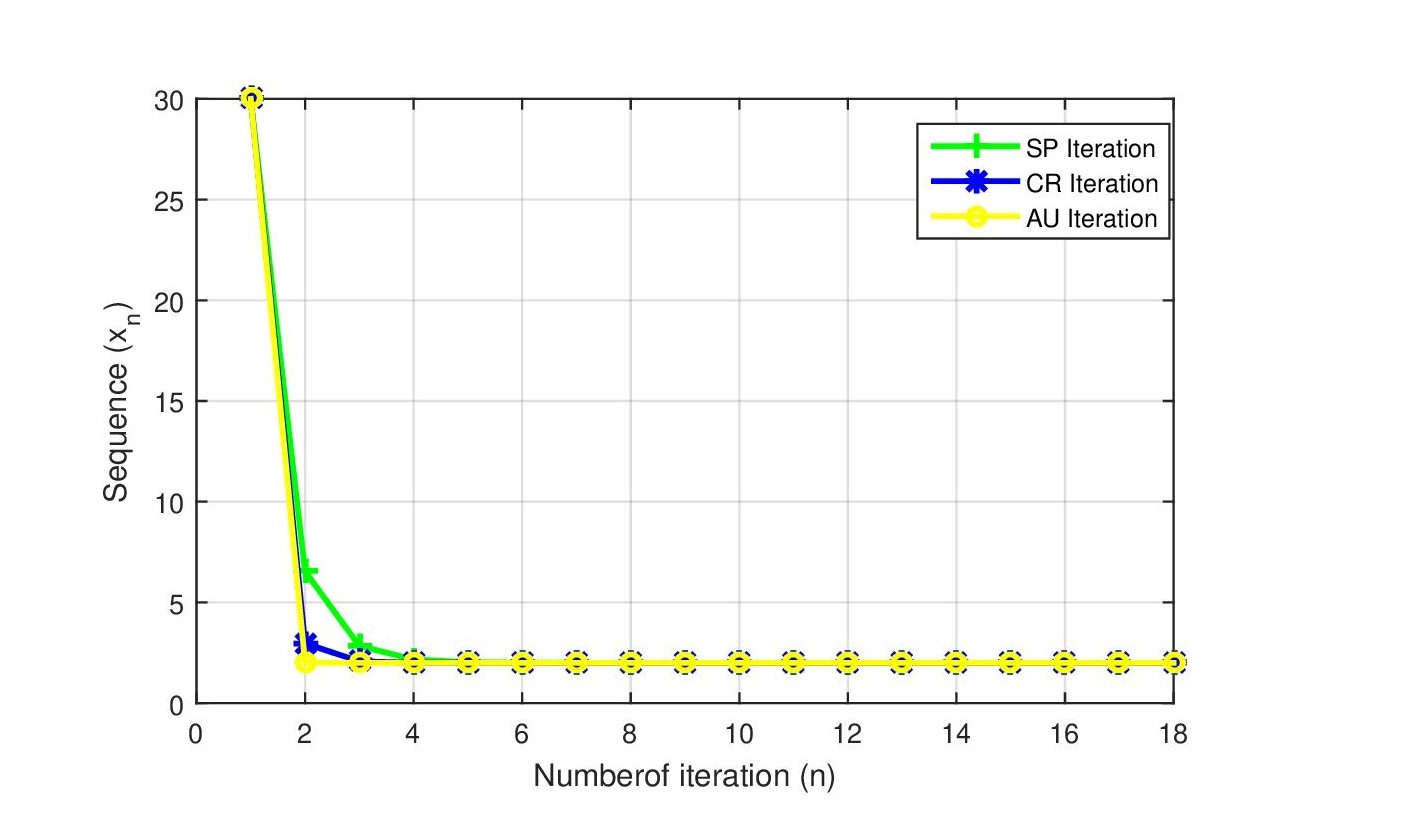
Table 3.A comparison of the different Iterative methods.

Step	SP	CR	AU
1	30.0000000000	30.0000000000	30.000000000
2	6.5399580891	2.9645498633	2.0055900713
3	2.8381224183	2.0693639599	2.0000025151
4	2.1634532374	2.0053107041	2.0000000011
5	2.0323255723	2.0004085862	2.0000000000
6	2.0064117448	2.0000314469	2.0000000000
7	2.0012725149	2.0000024204	2.0000000000
8	2.0002525810	2.0000001863	2.0000000000
9	2.0000501359	2.0000000143	2.0000000000
10	2.0000099517	2.0000000011	2.0000000000
11	2.0000019754	2.0000000001	2.0000000000
12	2.0000003921	2.0000000000	2.0000000000
13	2.0000000778	2.0000000000	2.0000000000
14	2.0000000154	2.0000000000	2.0000000000
15	2.0000000031	2.0000000000	2.0000000000
16	2.0000000006	2.0000000000	2.0000000000
17	2.0000000001	2.0000000000	2.0000000000
18	2.0000000000	2.0000000000	2.0000000000

From the above Tables and Figures, it is clear that AU iterative algorithm converges faster than a number of existing iterative algorithms.

6. Data dependence result

In this section, our focus is on the prove of data dependence result for fixed points of contraction mappings by utilizing AU iterative algorithm (12).

Theorem 11. Let \(\tilde{T}\) be an approximate solution of a contraction mapping \(T\). Let \(\{\psi_s\}\) be a sequence iteratively generated by AU iterative algorithm (12) and define an iterative algorithm \(\{\tilde{\psi_s}\}\) as follows:

where \(\{r_s\}\) is a sequence in \([0,1]\) satisfying the following conditions:

• (i) \(\frac{1}{2}\leq r_s,\,s\in\mathbb{N}\),
• (ii) \(\sum\limits _{s=0}^{\infty}r_s=\infty\).

If \(Tz=z\) and \(\tilde{T}\tilde{z}=\tilde{z}\) such that \(\lim\limits_{s\to\infty}\tilde{\psi}_s=\tilde{z}\), we have where \(\epsilon>0\) is a fixed number.

Proof. From (12) and (43), we have

Putting (45) into (46), we obtain Substituting (47) into (48), we have Putting (49) into (50), we obtain \begin{eqnarray} \nonumber\|\psi_{s+1}-\tilde{\psi}_{s+1}\|&\leq&\delta^4(1-(1-\delta)r_s)\|\psi_s-\tilde{\psi}_s\|+\delta^4 r_s\epsilon+\delta^3\epsilon+\delta^2\epsilon+\delta\epsilon+\epsilon. \label{e7}\end{eqnarray} Since \(r_s\in[0,1]\) and \(\delta\in[0,1)\), it implies that and using our assumption (i), we have \begin{eqnarray*} 1-r_s\leq r_s \Rightarrow 1=1-r_s+r_s\leq r_s+r_s=2r_s. \end{eqnarray*}From (51), we have Let \(\theta_s=\|\psi_{s}-\tilde{\psi}_{s}\|, \,\sigma_s=(1-\delta)r_s,\,\lambda_s=\frac{9\epsilon}{(1-\delta)}\), then from Lemma 7 and (52), we obtain Recalling Theorem 8, we have \(\lim\limits_{s\to\infty}\psi_s=z\) and from the assumption that \(\lim\limits_{s\to\infty}\tilde{\psi_s}=\tilde{z}\) together with (53) we have Hence, AU iterative algorithm (12) is data dependent. This completes the proof of Theorem 6.1

7. Application to a Volterra-Fredholm functional integral equation

In this section, we will use AU iterative algorithm (12) to find the solutions of a nonlinear integral equation.

Many problems of mathematical physics, applied sciences and engineering are reduced to Volterra-Fredholm integral equations (see for example, [21,22] and the references therein).

In 2011, Cracium and Serbian [23] considered and studied the following mixed-type Volterra-Fredholm functional nonlinear integral equation:

where \([u_1;v_1]\times\cdots\times[u_m;v_m]\) is an interval in \(\mathbb{\Re}^m\), \(K,H:[u_1;v_1]\times\cdots\times[u_m;v_m]\times[u_1;v_1]\times\cdots\times[u_m;v_m]\times \mathbb{\Re}\to \mathbb{\Re}\) continuous functions and \(F:[u_1;v_1]\times\cdots\times[u_m;v_m]\times\mathbb{\Re}^3\to\mathbb{\Re}\).

Recently, many authors in nonlinear analysis have constructed some iterative algorithms for approximating the unique solution of the mixed-type Volterra-Fredholm functional nonlinear integral equation (55) in Banach spaces (see for example, [24,25,26] and the references therein).

In this paper, we will prove the strong convergence of AU iterative algorithm (12) to the unique solution of the problem (55). The following theorem which was given by Cracium and Serbian [23] will be of great importance in proving our main results.

Theorem 12.[23] We assume that the following conditions are satisfied:

• (\(B_1\)) \(K,H\in \Gamma([u_1;v_1]\times\cdots\times[u_m;v_m]\times[u_1;v_1]\times\cdots\times[u_m;v_m]\times \mathbb{\Re})\);
• (\(B_2\)) \(F\in([u_1;v_1]\times\cdots\times[u_m;v_m]\times\mathbb{\Re}^3)\);
• (\(B_3\)) there exists nonnegative constants \(\alpha,\beta,\gamma\) such that \begin{eqnarray*} |F(t,f_1,\xi_1,h_1)-F(t,f_2,\xi_2,h_2)|\leq\alpha|f_1-f_2|+\beta|\xi_1-\xi_2|+\gamma|h_1-h_2|, \end{eqnarray*}for all \(t\in[u_1;v_1]\times\cdots\times[u_m;v_m]\), \(f_1,\xi_1,h_1,f_2,\xi_2,h_2\in\mathbb{\Re}\);
• (\(B_4\)) there exist nonnegative constants \(L_K\) and \(L_H\) such that \begin{eqnarray*} |K(t,\rho,f)-K(t,\rho,\xi)|\leq L_K|f-\xi|,\\ |H(t,\rho,f)-H(t,\rho,\xi)|\leq L_H |f-\xi|, \end{eqnarray*}for all \(t,\rho\in [u_1;v_1]\times\cdots\times[u_m;v_m],f,\xi\in\mathbb{\Re}\);
• (\(B_5\)) \(\alpha+(\beta L_K+\gamma L_H)(v_1-u_1)\cdots(v_m-u_m)< 1\). Then, the nonlinear integral equation (55) has a unique solution \(z\in C ([u_1;v_1]\times\cdots\times[u_m;v_m]).\)

We are now ready to prove our main result.

Theorem 13. Assume that all the conditions \((B_1)-(B_5)\) in Theorem 12 are satisfied. Let \(\{\psi_n\}\) be defined by AU iterative algorithm (12) with real sequence \(r_s\in[0,1]\), satisfying \(\sum\limits_{s=1}^{\infty}r_s=\infty\). Then (55) has a unique solution and the AU iterative algorithm (12) converges strongly to the unique solution of the mixed type Volterra-Fredholm functional nonlinear integral equation (55), say \(z\in C([u_1;v_1]\times\cdots\times[u_m;v_m])\).

Proof. We now consider the Banach space \(\Psi=C([u_1;v_1]\times\cdots\times[u_m;v_m],\|\cdot\|_C)\), where \(\|\cdot\|_C\) is the Chebyshev's norm. Let \(\{\psi_n\}\) be the iterative sequence generated by AU iterative algorithm (12) for the operator \(A:\Psi\to \Psi\) define by

Our intention now is to prove that \(\psi_s\to z\) as \(s\to \infty\). Now, by using (12), (55), (56) and the assumptions (\(B_1\))-\((B_5)\), we have that \begin{eqnarray} \nonumber \|g_s-z\|&=&\|A((1-r_s)\psi_s+r_sA\psi_s)-z\|\\ \nonumber &=&|A[(1-r_s)\psi_s+r_sA\psi_s](t)-A(z)(t)|\\ \nonumber&=&|F(t,[(1-r_s)\psi_s+r_sA\psi_s](t),\int_{u_1}^{q_1}\dots\\\nonumber&&\int_{u_m}^{q_m}K(t,\rho,[(1-r_s)\psi_s+r_sA\psi_s](\rho))d\rho,\int_{u_1}^{v_1}\dots\\\nonumber&&\int_{u_m}^{v_m}H(t,\rho,[(1-r_s)\psi_s+r_sA\psi_s](\rho))d\rho)\\&&\nonumber- F\left(t,z(t),\int_{u_1}^{q_1}\dots\int_{u_m}^{q_m}K(t,\rho,z(\rho))d\rho,\int_{u_1}^{v_1}\dots\int_{u_m}^{v_m}H(t,\rho,z(\rho))d\rho\right)|\\\nonumber \nonumber \end{eqnarray} \begin{eqnarray} \nonumber&\leq&\alpha|[(1-r_s)\psi_s+r_sA\psi_s](t)-z(t)|+\beta\int_{u_1}^{q_1}\dots\\\nonumber&&\int_{u_m}^{q_m}|K(t,\rho,[(1-r_s)\psi_s+r_sA\psi_s](\rho))-K(t,\rho,z(\rho))|d\rho\\&&\nonumber +\gamma\int_{u_1}^{v_1}\dots\int_{u_m}^{v_m}|H(t,\rho,[(1-r_s)\psi_s+r_sA\psi_s](\rho))-H(t,\rho,z(\rho))|d\rho \\ \nonumber&\leq&\alpha|[(1-r_s)\psi_s+r_sA\psi_s](t)-z(t)|+\beta\int_{u_1}^{q_1}\dots\\\nonumber&&\int_{u_m}^{q_m}L_K|[(1-r_s)\psi_s+r_sA\psi_s](\rho)-z(\rho)|ds\\&&\nonumber+\gamma\int_{u_1}^{v_1}\dots\int_{u_m}^{v_m}L_H|[(1-r_s)\psi_s+r_sA\psi_s](\rho)-z(\rho)|ds\\ \nonumber&\leq&\alpha\|(1-r_s)\psi_s+r_sA\psi_s-z\|+\beta \prod_{i=1}^{m}(v_i-u_i)L_K\|(1-r_s)\psi_s+r_sA\psi_s-p\|\\&&\nonumber+\gamma \prod_{i=1}^{m}(v_i-u_i)L_H\|(1-r_s)\psi_s+r_sA\psi_s-z\| \end{eqnarray} \begin{eqnarray} \nonumber \|(1-r_s)\psi_s&+&r_sA\psi_s-z\|\\\nonumber&\leq&(1-r_n)|\psi_s(t)-z(t)|+r_n|A(\psi_s)(t)-A(p)(t)|\\ \nonumber&=&(1-r_s)|\psi_s(t)-z(t)|\\&&\nonumber+r_s\left|F\left(t,\psi_s(t),\int_{u_1}^{q_1}\dots\int_{u_m}^{q_m}K(t,\rho,\psi_s(\rho))d\rho,\int_{u_1}^{v_1}\dots\int_{u_m}^{v_m}H(t,\rho,\psi_s(\rho))d\rho\right)\right.\\&&\left.\nonumber- F\left(t,\rho(t),\int_{u_1}^{q_1}\dots\int_{u_m}^{q_m}K(t,\rho,z(\rho))d\rho,\int_{u_1}^{v_1}\dots\int_{u_m}^{v_m}H(t,\rho,z(\rho))d\rho\right)\right| \end{eqnarray} \begin{eqnarray} \nonumber&\leq&(1-r_s)|\psi_s(t)-z(t)|+r_n\alpha|\psi_s(t)-z(t)|+r_s\beta\int_{u_1}^{q_1}\dots\int_{u_m}^{q_m}L_K|\psi_s(\rho)-z(\rho)|d\rho\\&&\nonumber+r_s\gamma\int_{u_1}^{v_1}\dots\int_{u_m}^{v_m}L_H|\psi_s(\rho)-z(\rho)|d\rho \end{eqnarray} Putting (59) into (58), we obtain From (12) and (60), we have \begin{eqnarray*} \nonumber \|k_{s}-z\|&=&\|Ag_s-z\|=|A(g_s)(t)-A(z)(t)|\\ \nonumber&=&\left|F\left(t,g_s(t),\int_{u_1}^{q_1}\dots\int_{u_m}^{q_m}K(t,\rho,g_s(\rho))d\rho,\int_{u_1}^{v_1}\dots\int_{u_m}^{v_m}H(t,\rho,g_s(\rho))d\rho\right)\right.\\&&\nonumber\left.- F\left(t,z(t),\int_{u_1}^{q_1}\dots\int_{u_m}^{q_m}K(t,\rho,z(\rho))d\rho,\int_{u_1}^{v_1}\dots\int_{u_m}^{v_m}H(t,\rho,z(\rho))d\rho\right)\right| \end{eqnarray*} \begin{eqnarray} \nonumber&\leq&\alpha|g_s(t)-z(t)|+\beta|\int_{u_1}^{q_1}\dots\int_{u_m}^{q_m}K(t,\rho,g_s(\rho))d\rho-\int_{u_1}^{q_1}\dots\int_{u_m}^{q_m}K(t,\rho,z(\rho))d\rho|\\&&\nonumber +\gamma|\int_{u_1}^{v_1}\dots\int_{u_m}^{v_m}H(t,\rho,g_s(\rho))d\rho-\int_{u_1}^{v_1}\dots\int_{u_m}^{v_m}H(t,\rho,z(\rho))d\rho|\\ \nonumber&\leq&\alpha|g_s(t)-z(t)|+\beta\int_{u_1}^{q_1}\dots\int_{u_m}^{q_m}|K(t,\rho,g_s(\rho))-K(t,\rho,z(\rho))|d\rho\\&&\nonumber +\gamma\int_{u_1}^{v_1}\dots\int_{u_m}^{v_m}|H(t,\rho,g_s(\rho))-H(t,\rho,z(\rho))|d\rho \\ \nonumber&\leq&\alpha|g_s(t)-z(t)|+\beta\int_{u_1}^{q_1}\dots\int_{u_m}^{q_m}L_K|g_s(\rho)-z(\rho)|d\rho+\gamma\int_{u_1}^{v_1}\dots\int_{u_m}^{v_m}L_H|g_s(\rho)-z(\rho)|d\rho \end{eqnarray} \begin{eqnarray} \nonumber&\leq&\alpha\|g_s-z\|+\beta \Pi_{i=1}^{m}(v_i-u_i)L_K\|g_s-z\|+\gamma \Pi_{i=1}^{m}(v_i-u_i)L_H\|g_s-z\|\\ \nonumber &=&[\alpha+(\beta L_K+\gamma L_H)\prod_{i=1}^{m}(v_i-u_i)]\|g_s-z\| \end{eqnarray} From (12) and (61), we have \begin{eqnarray} \nonumber \|\eta_{s}-z\|&=&\|Ak_s-z\|\\ \nonumber &=&|A(k_s)(t)-A(z)(t)|\\ \nonumber&=&|F\left(t,k_s(t),\int_{u_1}^{q_1}\dots\int_{u_m}^{q_m}K(t,\rho,k_s(\rho))d\rho,\int_{u_1}^{v_1}\dots\int_{u_m}^{v_m}H(t,\rho,k_s(\rho))d\rho\right)\\&&\nonumber- F\left(t,z(t),\int_{u_1}^{q_1}\dots\int_{u_m}^{q_m}K(t,\rho,z(\rho))d\rho,\int_{u_1}^{v_1}\dots\int_{u_m}^{v_m}H(t,\rho,z(\rho))d\rho\right)|\\\nonumber &\leq&\alpha|k_s(t)-z(t)|+\beta|\int_{u_1}^{q_1}\dots\int_{u_m}^{q_m}K(t,\rho,k_s(\rho))d\rho-\int_{u_1}^{q_1}\dots\int_{u_m}^{q_m}K(t,\rho,z(\rho))d\rho|\\&&\nonumber +\gamma|\int_{u_1}^{v_1}\dots\int_{u_m}^{v_m}H(t,\rho,k_s(\rho))d\rho-\int_{u_1}^{v_1}\dots\int_{u_m}^{v_m}H(t,\rho,z(\rho))d\rho|\\ \nonumber&\leq&\alpha|k_s(t)-z(t)|+\beta\int_{u_1}^{q_1}\dots\int_{u_m}^{q_m}|K(t,\rho,k_s(\rho))-K(t,\rho,z(\rho))|d\rho\\&&\nonumber +\gamma\int_{u_1}^{v_1}\dots\int_{u_m}^{v_m}|H(t,\rho,k_s(\rho))-H(t,\rho,z(\rho))|d\rho \\ \nonumber&\leq&\alpha|k_s(t)-z(t)|+\beta\int_{u_1}^{q_1}\dots\int_{u_m}^{q_m}L_K|k_s(\rho)-z(\rho)|d\rho+\gamma\int_{u_1}^{v_1}\dots\int_{u_m}^{v_m}L_H|k_s(\rho)-z(\rho)|d\rho \\ \nonumber&\leq&\alpha\|k_s-z\|+\beta \Pi_{i=1}^{m}(v_i-u_i)L_K\|k_s-z\|+\gamma \Pi_{i=1}^{m}(v_i-u_i)L_H\|k_s-z\|\\ \nonumber &=&[\alpha+(\beta L_K+\gamma L_H)\prod_{i=1}^{m}(v_i-u_i)]\|k_s-z\|\\ \end{eqnarray} Again, from (12) and (62), we obtain \begin{eqnarray*} \nonumber \|\eta_{s}-z\|&=&\|Ak_s-z\|=|A(k_s)(t)-A(z)(t)|\\ \nonumber \nonumber&=&\left|F\left(t,k_s(t),\int_{u_1}^{q_1}\dots\int_{u_m}^{q_m}K(t,\rho,k_s(\rho))d\rho,\int_{u_1}^{v_1}\dots\int_{u_m}^{v_m}H(t,\rho,k_s(\rho))d\rho\right)\right.\\&&\nonumber\left.- F\left(t,z(t),\int_{u_1}^{q_1}\dots\int_{u_m}^{q_m}K(t,\rho,z(\rho))d\rho,\int_{u_1}^{v_1}\dots\int_{u_m}^{v_m}H(t,\rho,z(\rho))d\rho\right)\right|\\\nonumber &\leq&\alpha|k_s(t)-z(t)|+\beta\left|\int_{u_1}^{q_1}\dots\int_{u_m}^{q_m}K(t,\rho,k_s(\rho))d\rho-\int_{u_1}^{q_1}\dots\int_{u_m}^{q_m}K(t,\rho,z(\rho))d\rho\right|\end{eqnarray*} \begin{eqnarray}&&\nonumber +\gamma\left|\int_{u_1}^{v_1}\dots\int_{u_m}^{v_m}H(t,\rho,k_s(\rho))d\rho-\int_{u_1}^{v_1}\dots\int_{u_m}^{v_m}H(t,\rho,z(\rho))d\rho\right|\\ \nonumber&\leq&\alpha|k_s(t)-z(t)|+\beta\int_{u_1}^{q_1}\dots\int_{u_m}^{q_m}|K(t,\rho,k_s(\rho))-K(t,\rho,z(\rho))|d\rho\\&&\nonumber +\gamma\int_{u_1}^{v_1}\dots\int_{u_m}^{v_m}|H(t,\rho,k_s(\rho))-H(t,\rho,z(\rho))|d\rho\\ \nonumber&\leq&\alpha|k_s(t)-z(t)|+\beta\int_{u_1}^{q_1}\dots\int_{u_m}^{q_m}L_K|k_s(\rho)-z(\rho)|d\rho+\gamma\int_{u_1}^{v_1}\dots\int_{u_m}^{v_m}L_H|k_s(\rho)-z(\rho)|d\rho \\ \nonumber&\leq&\alpha\|k_s-z\|+\beta \Pi_{i=1}^{m}(v_i-u_i)L_K\|k_s-z\|+\gamma \Pi_{i=1}^{m}(v_i-u_i)L_H\|k_s-z\|\\ \nonumber &=&[\alpha+(\beta L_K+\gamma L_H)\prod_{i=1}^{m}(v_i-u_i)]\|k_s-z\| \end{eqnarray} Finally, from (12) and (63), we obtain \begin{eqnarray} \nonumber \|\psi_{s+1}-z\|&=&\|A\eta_s-z\|\\ \nonumber &=&|A(\eta_s)(t)-A(z)(t)|\\ \nonumber \nonumber&=&\left|F\left(t,\eta_s(t),\int_{u_1}^{q_1}\dots\int_{u_m}^{q_m}K(t,\rho,\eta_s(\rho))d\rho,\int_{u_1}^{v_1}\dots\int_{u_m}^{v_m}H(t,\rho,\eta_s(\rho))d\rho\right)\right.\\&&\nonumber\left.- F\left(t,z(t),\int_{u_1}^{q_1}\dots\int_{u_m}^{q_m}K(t,\rho,z(\rho))d\rho,\int_{u_1}^{v_1}\dots\int_{u_m}^{v_m}H(t,\rho,z(\rho))d\rho\right)\right|\\\nonumber &\leq&\alpha|\eta_s(t)-z(t)|+\beta\left|\int_{u_1}^{q_1}\dots\int_{u_m}^{q_m}K(t,\rho,\eta_s(\rho))d\rho-\int_{u_1}^{q_1}\dots\int_{u_m}^{q_m}K(t,\rho,z(\rho))d\rho\right|\\&&\nonumber +\gamma\left|\int_{u_1}^{v_1}\dots\int_{u_m}^{v_m}H(t,\rho,\eta_s(\rho))d\rho-\int_{u_1}^{v_1}\dots\int_{u_m}^{v_m}H(t,\rho,z(\rho))d\rho\right|\\ \nonumber&\leq&\alpha|\eta_s(t)-z(t)|+\beta\int_{u_1}^{q_1}\dots\int_{u_m}^{q_m}|K(t,\rho,\eta_s(\rho))-K(t,\rho,z(\rho))|d\rho\\&&\nonumber +\gamma\int_{u_1}^{v_1}\dots\int_{u_m}^{v_m}|H(t,\rho,\eta_s(\rho))-H(t,\rho,z(\rho))|d\rho\\ \nonumber&\leq&\alpha|\eta_s(t)-z(t)|+\beta\int_{u_1}^{q_1}\dots\int_{u_m}^{q_m}L_K|\eta_s(\rho)-z(\rho)|d\rho+\gamma\int_{u_1}^{v_1}\dots\int_{u_m}^{v_m}L_H|\eta_s(\rho)-z(\rho)|d\rho \\ \notag&\leq&\alpha\|\eta_s-z\|+\beta \Pi_{i=1}^{m}(v_i-u_i)L_K\|\eta_s-z\|+\gamma \Pi_{i=1}^{m}(v_i-u_i)L_H\|\eta_s-z\| \\ \nonumber &=&[\alpha+(\beta L_K+\gamma L_H)\prod_{i=1}^{m}(v_i-u_i)]\|\eta_s-z\| \end{eqnarray} Since from condition (\(B_5\)) we have \([\alpha+(\beta L_K+\gamma L_H)\prod\limits_{i=1}^{m}(v_i-u_i)]< 1\), it follows that \( ([\alpha+(\beta L_K+\gamma L_H)\prod\limits_{i=1}^{m}(v_i-u_i)])^4 < 1\). Thus, (64) reduces to From (65), we have the following inequalities: From (66), we have Since \(r_n\in [0,1]\) for all \(n\in \mathbb{N}\) and recalling from assumption \((B_5)\) that \([\alpha+(\beta L_K+\gamma L_H)\prod_{i=1}^{m}(v_i-u_i)]< 1\), then we have From classical analysis, it is that \(1-\psi\leq e^{-\psi}\) for all \(\psi\in [0,1]\), thus from (67), we have Taking the limit of both sides of the above inequalities, we have \( \lim\limits_{s\to \infty}\|\psi_s-z\|=0\). Hence, (12) converges strongly to the unique solution of the mixed type Volterra-Fredholm functional nonlinear integral equation (55).

7. Conclusion

In this paper, we have proved that our new iterative algorithm (12) outperforms several well known iterative algorithms in the literature in terms of rate of convergence. The stability result of AU iterative algorithm has also been obtained. We have also shown that AU iterative algorithm (12) is data dependent. Finally, to illustrate the efficiently of AU iterative algorithm (12), we have proved approximated the unique solution of a nonlinear integral equation. Hence, our results are generalization and improvements of several well known results in the existing literature.

Author Contributions

All authors contributed equally to the writing of this paper. All authors read and approved the final manuscript.

Conflicts of Interest

''The authors declare no conflict of interest.''

References

Abass, H. A., Mebawondu, A. A., & Mewomo, O. T. (2018). Some results for a new three steps iteration scheme in Banach spaces.
Bulletin of the Transilvania University of Brasov. Mathematics, Informatics, Physics. Series III, 11(2), 1-18. [Google Scholor]
Mann, W. R. (1953). Mean value methods in iteration. Proceedings of the American Mathematical Society, 4(3), 506-510. [Google Scholor]
Ishikawa, S. (1974). Fixed points by a new iteration method. Proceedings of the American Mathematical Society, 44(1), 147-150. [Google Scholor]
Noor, M. A. (2000). New approximation schemes for general variational inequalities. Journal of Mathematical Analysis and Applications, 251(1), 217-229. [Google Scholor]
Agarwal, R. P., O Regan, D., & Sahu, D. R. (2007). Iterative construction of fixed points of nearly asymptotically nonexpansive mappings. Journal of Nonlinear and Convex Analysis, 8(1), 61-79. [Google Scholor]
Abbas, M., & Nazir, T. (2014). Some new faster iteration process applied to constrained minimization and feasibility problems. Matematicki Vesnik, 66, 223-234. [Google Scholor]
Phuengrattana, W., & Suantai, S. (2011). On the rate of convergence of Mann, Ishikawa, Noor and SP-iterations for continuous functions on an arbitrary interval. Journal of Computational and Applied Mathematics, 235(9), 3006-3014. [Google Scholor]
Karahan, I., & Ozdemir, M. (2013). A general iterative method for approximation of fixed points and their applications. Advances in Fixed Point Theory, 3(3), 510-526. [Google Scholor]
Chugh, R., Kumar, V., & Kumar, S. (2012). Strong convergence of a new three step iterative scheme in Banach spaces. American Journal of Computational Mathematics, 2(4), 345-357.[Google Scholor]
Sahu, D. R., & Petrusel, A. (2011). Strong convergence of iterative methods by strictly pseudocontractive mappings in Banach spaces. Nonlinear Analysis: Theory, Methods & Applications, 74(17), 6012-6023. [Google Scholor]
Gürsoy, F., & Karakaya, V. (2014). A Picard-S hybrid type iteration method for solving a differential equation with retarded argument. arXiv preprint arXiv:1403.2546.[Google Scholor]
Thakur, B. S., Thakur, D., & Postolache, M. (2016). A new iterative scheme for numerical reckoning fixed points of Suzuki’s generalized nonexpansive mappings. Applied Mathematics and Computation, 275, 147-155. [Google Scholor]
Ullah, K., & Arshad, M. (2018). Numerical reckoning fixed points for Suzuki’s generalized nonexpansive mappings via new iteration process. Filomat, 32(1), 187-196. [Google Scholor]
Ullah, K., & Arshad, M. (2017). New iteration process and numerical reckoning fixed points in Banach spaces. University Politehnica of Bucharest Scientific Bulletin Series A, 79(4), 113-122. [Google Scholor]
Garodia, C., & Uddin, I. (2020). A new fixed point algorithm for finding the solution of a delay differential equation. Aims Mathematics, 5(4), 3182-3200. [Google Scholor]
Thianwan, S. (2009). Common fixed points of new iterations for two asymptotically nonexpansive nonself-mappings in a Banach space. Journal of Computational and Applied Mathematics, 224(2), 688-695. [Google Scholor]
Berinde, V. (2004). Picard iteration converges faster than Mann iteration for a class of quasi-contractive operators. Fixed Point Theory and Applications, 2004, 716359. https://doi.org/10.1155/S1687182004311058. [Google Scholor]
Harder, A. M. (1987). Fixed Point Theory and Stability Results for Fixed Points Iteration Procedures [Ph. D. thesis]. University of Missouri-Rolla.[Google Scholor]
Weng, X. (1991). Fixed point iteration for local strictly pseudo-contractive mapping. Proceedings of the American Mathematical Society, 113(3), 727-731. [Google Scholor]
Soltuz, S. M., & Grosan, T. (2008). Data dependence for Ishikawa iteration when dealing with contractive-like operators. Fixed Point Theory and Applications, 2008, 242916. https://doi.org/10.1155/2008/242916. [Google Scholor]
Abdou, M. A., Nasr, M. E., & Abdel-Aty, M. A. (2017). Study of the normality and continuity for the mixed integral equations with phase-lag term. International Journal of Mathematical Analysis, 11(16), 787-799. [Google Scholor]
Abdou, M. A., Soliman, A. A., & Abdel-Aty, M. A. (2020). On a discussion of Volterra-Fredholm integral equation with discontinuous kernel. Journal of the Egyptian
Mathematical Society, 28(1), 1-10. [Google Scholor]
Craciun, C., & Serban, M. A. (2011). A nonlinear integral equation via Picard operators. Fixed point theory, 12(1), 57-70. [Google Scholor]
Garodia, C., & Uddin, I. (2018). Solution of a nonlinear integral equation via new fixed point iteration process. arXiv preprint arXiv:1809.03771. [Google Scholor]
Gürsoy, F. (2014). Applications of normal S-iterative method to a nonlinear integral equation. The Scientific World Journal, 2014, 943127. https://doi.org/10.1155/2014/943127. [Google Scholor]
Okeke, G. A., & Abbas, M. (2020). Fejér monotonicity and fixed point theorems with applications to a nonlinear integral equation in complex valued Banach spaces. Applied General Topology, 21(1), 135-158. [Google Scholor]