1Département de Mathématiques et Informatique (RDC), Faculté des Sciences, Université de Lubumbashi, Democratic Republic of the Congo.
2Département de Mathématiques, Informatique et Statistiques(RDC), Faculté des Sciences et Technologies, Université de Kinshasa, Democratic Republic of the Congo.
Stochastic differential equations (SDEs) are a powerful tool for modeling certain random trajectories of diffusion phenomena in the physical, ecological, economic, and management sciences. However, except in some cases, it is generally impossible to find an explicit solution to these equations. In this case, the numerical approach is the only favorable possibility to find an approximative solution. In this paper, we present the mean and mean-square stability of the Non-standard Euler-Maruyama numerical scheme using the Vasicek and geometric Brownian motion models.
In order to construct continuous and strongly Markovian processes whose generators are second-order differential operators called diffusions [1, 2], Ito developed stochastic differential equations, which are considered random perturbations added to ordinary differential equations or integral equations in which integrals are involved with respect to a Brownian motion. However, in general, finding explicit solutions for stochastic differential equations (SDEs), except in cases where diffusion and drift coefficients are linear, seems difficult or impossible [3].
This is why the numerical approach is relevant because there are numerical methods to predict in advance the qualitative behavior of solutions of stochastic differential equations such as stability. In this paper, we apply the approach described in [1, 4] to analyze the stability of the Vasicek and geometric Brownian motion models using the non-standard Euler-Maruyama scheme. At first glance, we present some basic concepts on the non-standard finite difference scheme of ordinary differential equations, the classical Euler-Maruyama scheme, and the non-standard scheme of SDEs.
2. Preliminaries notions
In this section, we present some important tools in connection with stochastic differential equations, stabilities, and numerical schemes, such as the Non-standard finite difference scheme, the Euler-Maruyama scheme, and the Non-standard Euler-Maruyama scheme.
2.1. Stochastic differential equation and stabilities
This section presents some definitions in connection with stochastic differential equations and the stabilities of solutions of SDEs.
Definition 1.(Stochastic differential equation (SDE), [5])
Let \(\left(\Omega,\mathcal{F},\left(\mathcal{F}_t\right)_{t\geq 0},\mathbb{P} \right)\) be a filtered probability space, \(\left(B_t\right)_{t\geq 0}\) a standard Brownian motion on \(\mathbb{R}^d\) defines in a filtered probability space. A stochastic differential equation (SDE) on \(\mathbb{R}^d \) is an equation of the form:
with the drift coefficient: \[b\left(t,X_t\right)\in \left[ 0,T\right] \times \mathbb{R}^n \longrightarrow \mathbb{R}^n\,,\] and the diffusion: \[\sigma \left(t,X_t\right)\in \left[ 0,T\right] \times \mathbb{R}^n \longrightarrow \mathbb{R}^{n\times d}\,,\] when \(X_o\) is random variable independent of \(\left(B_t\right)_{t\geq 0}\).
Remark 1.
The white noise \( \sigma \left(t,X_t\right) \) can be additive, it does not influence the state of the system.
The white noise \( \sigma \left(t,X_t\right) \) can be multiplicative, it’s influence the state of the system.
Theorem 1. (Existence and uniqueness [6])
We assume that there is a positive constant \( K \) such that \( \forall \quad t\geq 0\), \(X,Y \in \mathbb{R}^d\)
Linear growth condition: \[|b\left(t,X\right)|\leq K\left(1+|X|\right),\] \[|\sigma \left(t,X\right)|\leq K\left(1+|X|\right).\]
So the SDE \( \eqref{intelligent}\) admits, for any initial condition \(X_o\) of square integrable \(\left(E\left[|X_o|^2\right]< n\infty\right)\) the strong solution \(\left(X_t\right)_{t\in \left[0,T\right]}\), unique, almost surely continuous and satisfying the following condition:
\[ E\left(\underset{0\leq t\leq T}{\text{Sup}}|X_t^2|\right)<\infty\,.\]
According to [6] there exists one and only one solution for the Eq. \eqref{intelligent}, verifying the Lipschitz conditions.
Definition 2. (Asymptotic stability in probability in large sense [7])
The solution is said to be asymptotically and stochastically stable in the large sense if \[\forall \quad X_o \in \mathcal{L}^2_{\mathcal{F}_t}\left(\left[-T,0\right],\mathbb{R}^n\right),\] then
\[ \mathbb{P}\left\lbrace \underset{t\longrightarrow\infty}{\lim}X\left(t\right)=0\right\rbrace=1.\]
Definition 3. (Stability of \(p^{th}\) moment [1])
Let \(p\geq 2\) we say that a solution of \(\eqref{intelligent}\) is stable in \(p^{th}\) moment if \(\forall \epsilon>0\) it exists \(\delta>0\) such as
\[ E\left[ \underset{t>0}{\text{Sup}}|X\left(t\right)|^p \right]< \epsilon \text{ avec }|X_o|< \delta.\]
Let \(p\geq 2\), we say that a solution of \(\eqref{intelligent}\) is stable asymptoticaly in \(p^{th}\) moment if it is stable from \(p^{eme}\) moment \[\forall \quad X_o\in \mathcal{L}^2_{\mathcal{F}_{t_o}}\left(\left[-T,0\right],\mathbb{R}^n\right)\,,\] then we have
\[\underset{T\longrightarrow\infty}{\lim}E\left[ \underset{t> T}{\text{Sup}}|X\left(t\right)|^p \right]=0\,.\]
2.2. Numerical schemes of SDEs
In this section, we present two numerical schemes adapted to SDEs, firtly the Euler-Maruyama scheme and secondly the non-standard Euler-Maruyama scheme.
Definition 4.(Non-standard finite difference schemes [8, 9])
Let consider an ordinary differential equation whose general form is given by:
with \(X \in \mathbb{R}^{n}, f\in C^{2}(\mathbb{R}^{m},\mathbb{R}^{m})\).
Let \(I=[0,T]\) with \(T \in\mathbb{R}^+\) and \(\Delta t \in \mathbb{R} \forall \Delta t > 0\) for \(k \in \mathbb{N} \), we note \(t_k\) the discrete time defined as \(t_k=k\Delta t \) or \(\Delta t = \dfrac{t_k}{k}\).
A general numerical scheme of the non-standard type with one step \(\Delta t\) which approach the general solution of a system of the form \eqref{equa41} has the form:
\begin{equation*}
X_{k+1}=\phi({\Delta t })(X_k)=\phi({\Delta t ,X_k})\,,
\end{equation*}
when \(\phi({\Delta t })\) is \(C^2(\mathbb{R}^{m},\mathbb{R}^{m})\), \(X_k\) initial condition and \eqref{equa41} can be written as:
\begin{equation*}
\dfrac{dY}{dX} \simeq \dfrac{X_{k+1}-X_k}{\phi({\Delta t })}=f(X_k,X_{k+1},\Delta t)
\label{equa11}\,,
\end{equation*}
when
\begin{equation}\tag{3}
X_{k+1}=X_{k}+\phi({\Delta t }) f(X_k,X_{k+1},\Delta t) \,,
\end{equation}
with \[ \phi({\Delta t })=\Delta t + 0(\Delta t ^2 )\text{ and } \Delta t \longrightarrow 0\,. \]
Among the forms of the function \( \phi({\Delta t } )\) the most used form of the function \( \phi \) is of the form [1]6}:
\begin{equation*}
\phi({\Delta t })=\dfrac{1-e^{\lambda \Delta t}}{\lambda} \quad \forall \quad \lambda \in \mathbb{R}\,.
\label{equab}
\end{equation*}
Mickens in [11, 12, 13, 14] states five rules to be respected in order to build a good non-standard finite difference scheme.
An advantage of using this scheme is that issues related to consistency, stability and convergence do not appear. Let’s state the convergence of this scheme.
Definition 5.(Convergence of the Non-standard scheme [14]) A numerical scheme converges if the numerical solution \(X_k\) satisfies
\begin{equation*}
\sup_{0 \leq t_k \leq T} \|X_k-x( t_x ) \|\longrightarrow 0 , \Delta t \longrightarrow 0 \text{ et } x_{ 0} \longrightarrow x(t_0)\,.
\end{equation*}
It is of order \(p\) if
\begin{equation*}
\sup_{0 \leq t_k \leq T} \|X_{x}-x( t_x ) \|_{\infty}= 0 , (\Delta t)^p+0+\left( \|X_{x}-x(\Delta t ) \|\right)\,,
\end{equation*}
when \(\Delta t \longrightarrow 0 \text{ and } x_{0} \longrightarrow x(t_0)\).
Let us consider another improving definition of Mickens on the non-standard finite difference scheme according to Lubuma and Anguelov:
Definition 6.(DFNS according to Lubuma and Anguelov [15, 16])
A general one-step numerical scheme that approximates the solution of \eqref{equa41} is said to be a non-standard finite difference scheme if at least one of the following conditions is satisfied:
\(\displaystyle {\frac{d}{dx}X(t_k)\approx \frac{X_{k+1}-X_k}{\phi{(\Delta t) }}} \) with \(\phi({\Delta t }) = \Delta t + 0(\Delta t )^2\) is a positive function.
The nonlocal approximation of \(f(t_k,X(t_k))\) is \(\phi_{\Delta t }(f,X_k)=\overline{\phi}_{\Delta t }(f,X_k,X_{k+1})\).
Definition 7.(Euler-Maruyama scheme [5, 17])
Let \(\{X_{t}\}\) be the diffusion solution of the SDE \eqref{intelligent}. Let us consider the interval \([0,T]\) and a regular subdivision: \[t_{0}=0< t_{1}< t_{2}< t_{0}< \cdots< t_{k}=T \quad \text{with step}\quad \Delta t=\frac{T}{N}=\frac{T}{k}.\]
The Euler-Maruyama scheme of \(\eqref{intelligent}\) is defined as:
Let us now state the definition of the non-standard Euler-Maruyama scheme based on the definitions of the non-standard finite difference scheme and the Euler-Maruyama scheme discussed earlier.
Definition 8.(Non-standard Euler-Maruyama scheme [14,18])
Considering the non-standard scheme definition rules, we define the Non-standard Euler-Maruyama scheme (EMNS) applied to \(\eqref{intelligent}\) and \eqref{snum2} which is given by:
with \(\phi(\Delta t) = \Delta t + C(\Delta t)\), a positive function of \( \Delta t \) and \(\Delta B_k = B_{k+1}-B_k .\)
In the following subsection, we present some elements of the construction of this scheme, including convergence.
[\(H_1\)] For the initial condition, we assume that it is chosen independently of the Brownian motion \(B_t\) of the Eq. \eqref{equa417}.
[\(H_2\)] The local Liptschitz condition i.e. \(\forall \;R> 0 ~\exists L_R\) depends on \(R\) such us
\begin{equation*}
\left| b(x)-b(y)\right| \vee \left| \sigma(x)-\sigma(y)\right| \leq L_R \left| x-y\right| \quad x,y \in \mathbb{R}^n
\end{equation*} with \(\left| x\right|\vee \left| y\right| \leq R\).
[\(H_3\)] Linear growth condition
\(~\exists \;k> 0\) such that
\begin{equation*}
\left| b(x)\right| \vee \left| \sigma(x)\right| \leq k(1+\left| x\right| )\quad \forall x \in \mathbb{R}^n\,.
\end{equation*}
Let us consider another result useful concerning the convergence of the non-standard Euler-Maruyama scheme.
Theorem 3.(Strong convergence of the NSEMS [18])
Under assumptions \(H_1\), \(H_2\) and \(H_3\), for any \(p \geq 2\) there exists a constant \(c_1\) depending only on \(\delta t\) and \(p\) such that the exact solution of the approximation given by the non-standard Euler-Maruyama scheme of \eqref{equa417} have the following property:
\begin{equation*}
E\left[ \sup_{0\leq t \leq T} \left| Y_t\right|^p\right] \vee E\left[ \sup_{0\leq t \leq T} \left| {X}^{EMNS}(t)\right|^p\right] \leq c_1(\Delta t, p)\,,
\end{equation*}
the solution obtained with the non-standard Euler-Maruyama scheme scheme of \eqref{equa417} is strongly convergent.
The remaining paper is organized as follows. In S3, non-standard Euler-Maruyama asymptotic stability in mean and mean-square for Vasicek and Geometric Brownian motion is carried out and classical proof will be given for each case. Finally, in S4, numerical investigations and residual calculations are provided and discussed.
3. Non-standard Euler-Maruyama stabilities
In this section we will consider two models of SDEs; the first SDE model, of Vasicek, involves white noise of an additive nature, while the second model, the geometric Brownian motion, is of multiplicative type. Let consider the first, the Vasicek model.
3.1. Vasicek model
Let’s consider the following SDE representing the Vasicek model [1]:
Considering the solution of \eqref{equa(2)}, the mean and the mean-square give respectively:
\begin{equation*}
E[\left| X_t\right| ] = \frac{\theta_1}{\theta_2}\,,
\end{equation*}
and
\begin{equation*}
E(\left| X_t\right|^2) = \frac{\theta^2_3}{2\theta_2}\,. \end{equation*}
Which means that the stochastic process \[X_t \simeq \mathcal{N}\left( \frac{\theta_1}{\theta_2},\frac{\theta^2_3}{2\theta_2}\right) \,.\]
By using some properties of Brownian motion, the solution of the model \eqref{equa(2)} can be written as follows:
Now, we present some numerical stabilities conditions for the system \eqref{eq(1)} of non-standard scheme and the proofs of these based on the approach described in [4] and used in [1].
The Euler-Maruyama scheme associated with \eqref{eq(1)} is:
\begin{equation*}
\begin{aligned}
X^{EM}_{k +1} & = X_k + (\theta_1 – \theta_2 X_k)\Delta t_k + \theta_3 \Delta B_k.
\end{aligned}
\end{equation*}
After calculation, we get
\begin{equation}\tag{9}
X^{EM}_{k +1} =\theta_1 \Delta t + (1 – \Delta t \theta_2)X_k + \theta_3 \sqrt{\Delta t}Z_k.
\label{eq(2)}
\end{equation}
Remark 2.We assume that the variable follows the normal distribution of expectation \(0\) and mean-square \( 1\). i.e., \[Z_k \simeq \mathcal{N}(0,1)\,.\]
The non-standard Euler-Maruyama scheme associated to \eqref{eq(2)} is
\begin{equation*}
\begin{aligned}
X^{EMNS}_{k +1} &= X_k + (\theta_1 – \theta_2X_k)\phi(\Delta t) + \theta_3 \Delta B_k
= X_k + \theta_1\phi( \Delta t) – \theta_2\phi(\Delta t)X_k + \theta_3 \Delta B_k\,.
\end{aligned}
\end{equation*}
After calculation, we obtain
Remark 3.
The positive function, \(\phi(\Delta t)\) is calculated using the procedure described by Mickens in [20]. In the framework of this stochastic differential equation of Vasicek, we consider only the part containing the drift \(b\) for the computed, i.e., \( b(t,X_t) = (\theta_1 – \theta_2X_t)dt\,, \) and the part containing the diffusion \(\sigma\), i.e., \( \sigma (t,X_t)= \theta_3dB_t \) remains unchanged.
After determination of the function \( \phi{(\Delta t)} \), while respecting the rules described in [20], the function \( \phi(\Delta t)\) gives:
Let us analyse the numerical mean and mean-square stabilities of the Non-standard Euler-Maruyama scheme of the Vasicek stochastic differential equation model.
3.1.1. Mean stability of non-standard Euler-Maruyama scheme
Theorem 4.[Mean stability of non-standard Euler-Maruyama scheme]
The non-standard Euler-Maruyama scheme of the model \eqref{eq(1)} is asymptotically stable in mean if
\begin{equation*}
E\left( X^{EMNS}_{k+1}\right) = \left| e^{-\theta_2 \Delta t}\right| ^{k+1}E\left( X_0\right) + \left| \frac{3\theta_1}{2\theta_2}(1-\frac{1}{3}e^{-\theta_2 \Delta t})\right| \left( 1+\sum_{i=1}^{k+1}\left| e^{-\theta_2 \Delta t}\right| ^i\right) \label{eq(5)}\,,
\end{equation*}
with \(
\left| e^{-\theta_2 \Delta t}\right| < 1
\) and
\(
\lim_{\Delta t \to 0} \left( \lim_{x \to \infty}E\left( X^{EMNS}_{k+1}\right) \right) = \frac{\theta_1}{\theta_2}.
\)
and just as in the case of \(I_2 = \left| \frac{3\theta_1}{2\theta_2}(1 – \dfrac{1}{3}e^{-\theta_2\Delta t})\right| \displaystyle\left( 1+\sum_{i = 1}^{k + 1}|e^{-\theta_2 \Delta t}|^i\right) \) as \(\Delta t \to 0\) and \(\theta_2 > 0\) with \(\left| e^{-\theta_2 \Delta t}\right| < 1\), then we have that
Theorem 6.
Under the assumptions, the non-standard Euler-Maruyama scheme in mean and mean-square is asymptotically stable if we have respectively \( \left|e^{-\theta_2 \Delta t}\right| < 1\) and \( \left|1- e^{-\theta_2 \Delta t}\right| 0.\)
Let’s consider the second model, the Geometric Brownian motion.
3.2. Geometric Brownian motion
Consider the following stochastic differential equation [1], describing geometric Brownian motion
The the right hand variable, follows a normal distribution, it can also be written in the form:
\begin{equation*}
X_t = X_s e^{\left\lbrace \left( \theta_1-\frac{1}{2}\theta_2^2\right) t + \theta_2 \left( B_t -B_s\right) \right\rbrace }\label{6c}
\,.\end{equation*}
The mean and the mean-square of \eqref{6b} give respectively:
For mean, if \(t\to \infty\) and \(\theta_1 < 0\), we have
\begin{equation*}
\lim_{t \to \infty}E(X_t) = \lim_{k \to \infty} X_0 e^{\theta_1 t} = 0
\,.\end{equation*}
For mean-square, if \(\left( 2\theta_1+\theta_2^2\right)< 0\) and \(t \to \infty\) i.e.,
\begin{equation*}
\lim_{t \to \infty}E(X_t^2) = 0 \text{ with } \left( 2\theta_1+\theta_2^2\right)< 0.
\end{equation*}
The Euler-Maruyama scheme of the geometric Brownian motion model [1] associated with \eqref{eq(7)} is
with \(\Delta B_k = \sqrt{\Delta t} Z_k,\) and \(Z_k \simeq \mathcal{N}(0,1).\)
The non-standard Euler-Maruyama scheme associated to \eqref{eq(8)} is
\begin{equation*}
X^{EMNS}_{k+1} = X_k + \theta_1 \phi (\Delta t) X_k + \theta_2 X_k \Delta B_k
\,.\end{equation*}
After some calculations, we get
Remark 5.
Given, the nature of the function \(\phi(\Delta t)\), a positive function. In the framework of the stochastic differential equation of geometrical Brownian motion that we treat, to calculate the function \( \phi(\Delta t)\), we consider only the part containing the drift \( b(t,X_t) = \theta_1X_tdt\) and the part containing the diffusion \( \sigma (t,X_t)= \theta_2X_tdB_t\) remains unchanged.
Calculating \(\phi(\Delta t)\) without diffusion according to [20], we have
Let us evaluate the stabilities of the expression \eqref{eq(11)}.
In the following paragraph, we state and prove the mean and mean-square stability conditions of the Non-standard Euler-Maruyama scheme. Let us start with the mean stability of the scheme.
3.2.1. Mean stability of the non-standard Euler-Maruyama scheme
Theorem 7.(Mean stability of the non-standard Euler-Maruyama scheme)
The non-standard Euler-Maruyama scheme of the model \eqref{eq(7)} is asymptotically stable in mean if
\begin{equation*}
E\left( X^{EMNS}_{k+1}\right) = \left( e^{\theta_1\Delta t}\right)^{k+1} E\left( X_0\right)\,, \label{eq(12)}
\end{equation*}
with \( \left| e^{\theta_1 \Delta t}\right| < 1 ;\quad \theta_1< 0 \) and
\begin{equation*}
\lim_{\Delta t \to 0} \left( \lim_{x \to \infty}E\left( X^{EMNS}_{k+1}\right) \right) = 0\,.
\end{equation*}
Proof.
Let’s calculate the mean of the non-standard Euler-Maruyama scheme.
\[\begin{aligned}
E\left( X^{EMNS}_{k+1}\right) &= E\left[ \left( e^{\theta_1\Delta t}+\theta_2 \sqrt{\Delta t}Z_k\right) X_k\right] \\
&= E\left( e^{\theta_1\Delta t}X_k\right) + E\left( \theta_2 \sqrt{\Delta t}X_k\right)E\left( Z_k\right) \quad \text{avec} \quad E\left( Z_k\right)=0\\
&= e^{\theta_1\Delta t} E\left( X_k\right)\\
&= e^{\theta_1\Delta t}\left( e^{\theta_1\Delta t}\left( e^{\theta_1\Delta t}\left( e^{\theta_1\Delta t}\left( \cdots e^{\theta_1\Delta t}E\left( X_0\right)\right) \right) \right) \right)\,.
\end{aligned}\]
Continuing with the iterations, we get
$$\tag{22}
E\left( X^{EMNS}_{k+1}\right) = \left( e^{\theta_{1}\Delta t}\right)^{k+1} E \left( X_{0}\right).
$$
If we assume that \[ \left| e^{\theta_1 \Delta t}\right| < 1 \quad \text{with} \quad \theta_1 < 0 , \] passing to the limit for \( \Delta t \to 0 \) and \( k \to +\infty \) we get the sought result i.e.,
\begin{equation*}
\lim_{\Delta t \to 0} \left( \lim_{x \rightarrow \infty}E\left( X^{EMNS}_{k+1}\right) \right) = 0\,.
\end{equation*}
%
3.2.2. Mean-square stability of the non-standard Euler-Maruyama scheme
Theorem 8.(Mean-square stability of the EMNS scheme)
The non-standard Euler-Maruyama scheme of the model \eqref{eq(7)} is asymptotically stable in mean-square if
\begin{equation*}
E\left( \left| X^{EMNS}_{k+1}\right|^2 \right) = \left( \left( e^{\theta_1\Delta t}\right) +\left( \left| \theta_2 \sqrt{\Delta t}\right| \right)\right)^{2(k+1)}\left( E\left| X_{0}\right| ^2\right)\,,
\end{equation*}
with
\begin{equation*}
\left| e^{\theta_1\Delta t}+ \theta_2 \sqrt{\Delta t}\right| < 1\,,
\end{equation*}
and
\begin{equation*}
\lim_{\Delta t \to 0} \left( \lim_{x \to \infty}E\left( X^{EMNS}_{k+1}\right) \right) =0\,.
\end{equation*}
If we assume that \[\left| e^{\theta_1\Delta t}+ \theta_2 \sqrt{\Delta t}\right| < 1 \] from the fact that the sequence is geometric, going to the limit with the fact that the quantity \[ E\left(\left| X^{EMNS}_{k+1}\right| \right) = 0 \,.\] For \( \Delta t \to 0 \) and \( k \to +\infty ,\) we find that
\begin{equation*}
\lim_{\Delta t \to 0} \left( \lim_{x \to \infty}E\left( X^{EMNS}_{k+1}\right) \right) =0.
\end{equation*}
Theorem 9.
Under the assumptions, the non-standard Euler-Maruyama scheme in mean and mean-square is asymptotically stable if \[\left| e^{\theta_1 \Delta t}\right| < 1 \quad \text{with} \quad \theta_1 0\]
respectively
\[\left| e^{\theta_1\Delta t}+ \theta_2 \sqrt{\Delta t}\right| < 1.\]
4. Numerical simulations of the models
This section presents some numerical simulations of Vasicek and geometric Brownian motion models. We treat the stability and instability cases and the increasing and decreasing cases. We will associate with each model the calculation of the residuals.
Let’s start with the simulation of the first model, the Vasicek’s one.
4.1. Vasicek model simulation
In this subsection, we consider the Vasicek equation, we present the different simulations of this model.
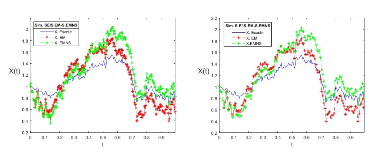
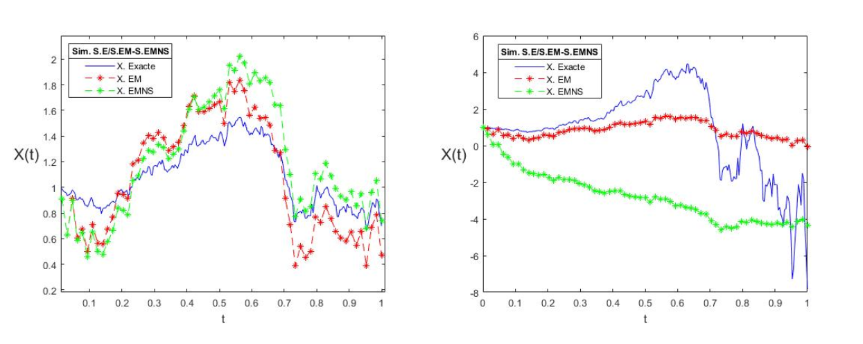
Figure 1. Stability of the Vasicek model using the EMNS scheme.Figure 2. Stability and instability of the Vasicek model using the EMNS scheme.
4.2. Geometric Brownian motion model simulation
In this subsection, we present the different numerical simulations of geometric Brownian motion.
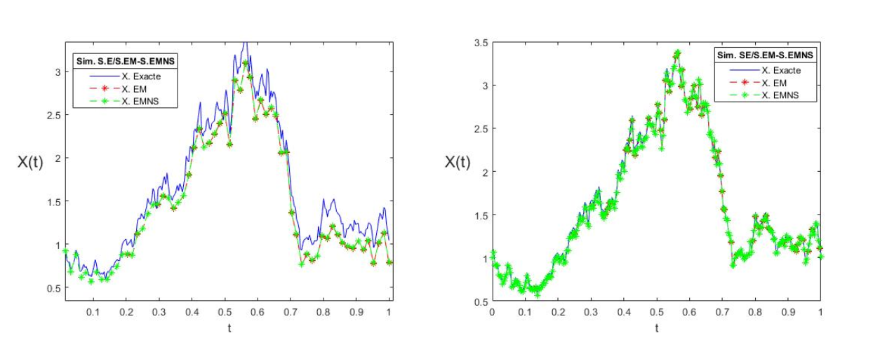
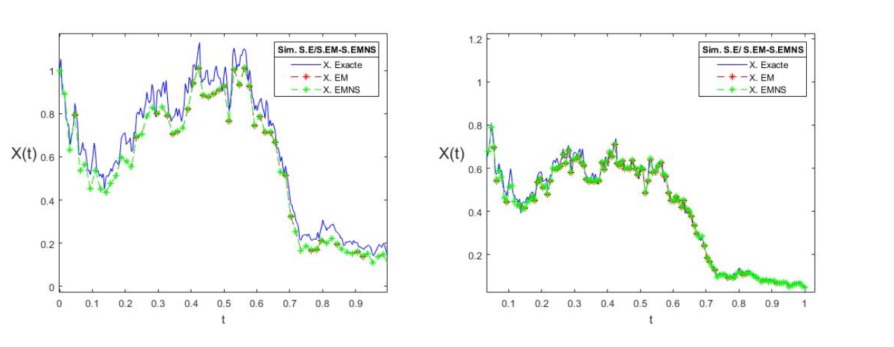
Figure 3. Increasing case of geometric Brownian motion.Figure 4. decreasing case of geometric Brownian motion.
4.3. Interpretations of the results
4.3.1. Vasicek’s Model
The two figures in Figure 1 show that there is stability of the non-standard Euler-Maruyama scheme for the Vasicek model. Moreover, the errors are smaller, namely \(\text{Emnserr} = 0.0338\) resp. (\(\text{Emnserr} = 0.0354\)) compared to the errors obtained by using the Euler-Maruyama scheme \(\text{Emerr} = 0. 2280\) resp. (\(\text{Emerr} = 0.2286\)) of the same model for a \(\Delta t=0.004\) resp.( \(\Delta t=0.015\)).
On the other hand the two other figures in Figure 2 show that there is stability resp.(instability) of the non-standard Euler-Maruyama scheme for the Vasicek model, because the errors are smaller namely \(\text{Emnserr} = 0. 0377\) resp. (\(\text{Emnserr} = 3.4794\)) compared to those obtained with the Euler-Maruyama scheme \(\text{Emerr} = 0.2298\) resp. (\(\text{Emerr} = 7.7772\)) of the same model for a \(\Delta t=0.015\).
Although the same discretization step was considered, the instability is because the value of the parameter \( \theta_2 =-4\) i.e., negative, does not correspond to the right value for this parameter.
4.3.2. Geometric Brownian motion model
The two figures, i.e., Figure 3 and Figure 4 present the stability of the model of geometric Brownian motion; the first two figures in Figure 3 are elaborated with a positive \( \theta_1 \) that is why the figures express the growth while in the two figures of Figure 4 with a negative \( \theta_1 \) that is why the figures express the decrease.
However, in both figures in Figure 3 the errors are smaller i.e. \(\text{Emnserr} = 0.2548\) respectively (\(\text{Emnserr} = 0. 0283 \) ) compared to the Euler-Maruyama scheme \(\text{Emerr} = 0.2611\) resp. (\(\text{Emerr} = 0.0303\)) of this model for a \(\Delta t=0.015\) resp. \((\Delta t=0.004 )\) for a \( \theta_1=1\).
On the other hand, in the two other figures of Figure 4 the errors of the non-standard Euler-Maruyama scheme are smaller \(\text{Emnserr} = 0.0415\) resp. (\(\text{Emnserr} =0. 0046 \)) compared to the errors obtained with the Euler-Maruyama scheme \(\text{Emerr} =0.0423 \)) resp. (\( \text{Emerr} = 0.0054 \)) for a \( \Delta t=0.015\) resp.(\( \Delta t= 0.008\)) for a \( \theta_1=-1 \) resp.(\( \theta_1=-2 \)).
Remark 6.
In line with the results obtained in the residual calculations for the two stochastic differential equation models treated, we find that the non-standard Euler-Maruyama scheme is better than the Euler-Maruyama scheme, as the latter improves on the Euler-Maruyama scheme by best approximating the exact solutions.
5. Conclusion
This paper presents the mean and mean-square stability of the non-standard Euler-Maruyama scheme using Vasicek and the geometric Brownian motion models. Both models are linear in dimension one; the Vasicek model is additive noise while the geometric Brownian motion is of multiplicative type; In these models we have established the conditions of numerical stabilities of the Non-standard Euler-Maruyama scheme, and a comparison has been made with the Euler-Maruyama scheme.
These conditions are stated as theorems, and we prove these results using the classical approach. The results found were supported by numerical simulations and the determination of residuals. It should be noted that the Non-standard Euler-Maruyama scheme improves the Euler-Maruyama scheme. In future work, we will focus on a Non-standard scheme of non-linear and higher dimensional SDEs.
Acknowledgments :
The authors would like to thank the referee for his/her valuable comments that resulted in the present improved version of the article.
Conflicts of Interest:
”The author declares no conflict of interest.”
Data Availability:
All data required for this research is included within this paper.
Funding Information:
No funding is available for this research.
References
Badibi, O.C., Ramadhani,I., Ndondo, M.A. & Kumwimba, S.D. (2023). Numerical stabilities of Vasicek and Geometric Brownian motion models.European Journal of Mathematical Analysis, 3, Article No. 8.[Google Scholor]
Richard, J. P. (2002).Mathématiques pour les systémes dynamiques. Hermés Science Publication, Paris, Paris.
Ahmad, R. (1988).Introduction to Stochastic Differential Equations. M Dekker, 1988. [Google Scholor]
Saito, Y. (2008). Stability analysis of numerical methods for stochastic systems with additive noise.Review of Economics and Information Studies, 8(3-4), 119-123. [Google Scholor]
Øksendal , B., & Sulem, A. (2005).Stochastic Control of Jump Diffusions(pp. 39-58). Springer Berlin Heidelberg.[Google Scholor]
Lyapunov, A. M. (1892). A general task about the stability of motion.Ph. D. Thesis, University of Kazan, Tatarstan (Russia).[Google Scholor]
Mickens, R. E., & Washington, T. M. (2012). A note on an NSFD scheme for a mathematical model of respiratory virus transmission.Journal of Difference Equations and Applications, 18(3), 525-529.[Google Scholor]
Mickens, R. E. (2005).Advances in the Applications of Nonstandard Finite Difference Schemes. World Scientific.[Google Scholor]
Mickens, R. E. (1994).Nonstandard Finite Difference Models of Differential Equations. world scientific.[Google Scholor]
Mickens, R. E. (2005). Discrete models of differential equations: the roles of dynamic consistency and positivity. InDifference Equations and Discrete Dynamical Systems (pp. 51-70).[Google Scholor]
Mickens, R. E. (2007). Numerical integration of population models satisfying conservation laws: NSFD methods.Journal of Biological Dynamics, 1(4), 427-436.[Google Scholor]
Mickens, R. E. (2000).Applications of nonstandard finite difference schemes. World Scientific.[Google Scholor]
Pierret, F. (2015). Modélisation de systèmes dynamiques déterministes, stochastiques ou discrets: application à l’astronomie et à la physique (Doctoral dissertation, Observatoire de Paris).
[Google Scholor]
Anguelov, R., & Lubuma, J. M. S. (2000).On the nonstandard finite difference method.Notices of the South African Mathematical Society, 31, 143-152.[Google Scholor]
Anguelov, R., & Lubuma, J. M. S. (2001). Contributions to the mathematics of the nonstandard finite difference method and applications.Numerical Methods for Partial Differential Equations: An International Journal, 17(5), 518-543.[Google Scholor]
Kloeden, P. E., & Platen, E. (1992). Stochastic differential equations. InNumerical Solution of Stochastic Differential Equations (pp. 103-160). Springer, Berlin, Heidelberg.[Google Scholor]
Platen, E., & Bruti-Liberati, N. (2010). Numerical Solution of Stochastic Differential Equations with Jumps in Finance (Vol. 64). Springer Science & Business Media.[Google Scholor]
Cresson, J., & Pierret, F. (2016). Non standard finite difference scheme preserving dynamical properties.Journal of Computational and Applied Mathematics, 303, 15-30.[Google Scholor]
Mickens, R. E. (2007). Calculation of denominator functions for nonstandard finite difference schemes for differential equations satisfying a positivity condition. Numerical Methods for Partial Differential Equations: An International Journal, 23(3), 672-691. [Google Scholor]