1University of Management and Technology, Lahore-54770, Pakistan.
2Department of Artificial Intelligence method and Applied Mathematics in the Faculty of Computer Science and Information Technology, West Pomeranian University of Technology, Szczecin, 71-210, Poland.
In 1965, L.A Zadeh inaugurated the idea of fuzzy set theory by extrapolating classical set theory. Later, Atanassov popularized it as an intuitionistic fuzzy set (IFS) more precisely than the fuzzy logic theory in 1983. IFS is highly fruitful in expounding uncertain situations which we face in decision making. In this paper, we have reexamined the idea of IFS and suggested the applications in decision making methods. Moreover, this theory helps us find the solution of one-shot decision (OSD) problems we mostly face in trade and economics, and the behavior of the decision person and assists them to get the best answer.
Decision theory throws light on decisions. Though we observe a little unification in this theory but a wide range of approaches to promote it is also found. For instance, expected utility (Probability weighted theory) and their types, probability and possibility theory. But the possibility distribution is the appropriate theory. Nevertheless, all these theories are based on lottery which generally comply the Bernoullian frame-work of the weighted average [1].
One-shot decision is exemplary condition wherever a person has simply unique opportunity for a judgement. Here are some examples that can enhance the concept of decision and abstract issues. Shall I take the umbrella with me? But I have no idea whether it will rain or not, so the decision depends on something about which I have no idea. I want to buy a house for 100000 but at the same time, another house which is much better than this in the same price attracts me. Should I continue with my search for another house or be contented with it? I am a smoker, one cigarette can satisfy me. Should I smoke another cigarette in this condition neglecting the harm? Decision plays a vital role in every act of a human being. Therefore, a theory about decision almost resembles with the theory of human activities.
A decision making condition has many factors, i.e. alternatives are usually modes of action that a person makes when he decides for something. And it totally depends on the choice of an alternative as well as on the elements which are beyond his reach. Sometimes, in a limiting case a decision maker does not know which state of nature will take place. Then it is easy to make a choice because the result of each alternative is sure to happen otherwise a decision maker acts under uncertainty [2]. Non-certainty is divided into three classes: risk, uncertainty and ignorance.
The risk involves in those situations when the chances of all possible results can be precisely obtained. Non-certainty conditions are linked with the little knowledge when chance cannot be exactly obtained [3]. Ignorance takes place when no information is obtainable to differentiate which state of nature is sure to take place.
It is observed that when we make a decision promptly, its effect doubtlessly is lasting though we have to face such decisions in trade and economics [4]. In OSD theory, keeping focus point in view, a decision maker always makes decisions. There are two things which should be kept in mind regarding OSD theory. Firstly, a person tries to find out what focus points should be considered for each alternative among all the focus points. Secondly, a person measures alternatives totally depending on focus arguments. The connection between various focus points is examined, and the result of these focus points(decision points) demonstrate the various aspects of a decision maker. Among these, the focus points, like active, passive, apprehensive and daring are the prominent ones.
It can be inferred that decision theories under uncertainty are highly linked with the option that is based on lottery. But here are some issues which we faced in OSD theory. For example, does the probability distribution rightly portray the uncertainty? The answer is that the probability gives us the option behind the occurrence of a specific event. In probability distribution lottery technique is one of the way, this technique defines the chance of a happening[1, 5]. The assumption of possibility [2, 6] portrays the uncertainty theories in which we are unable to find the optimal decision. The optimistic as well as pessimistic theories [7, 8] are helpful in making a decision and retaken for granted. Giang and Shenoy [9] popularized them with the help of standard draws. Moreover, these decision theories deal with the option based on uncertainty and its objectives are possibility distribution, expected utility, subjective expected utility and their kinds, and set up regarding profit and loss [10]. As a matter of fact, these are different theories for various decision conditions. But one shot decision theory is quite suitable in the condition where a choice is experienced just once.
It has been observed that people take decision making arduous due to fear of the incorrect decision [11]. The theory of IFS can be useful in this kind of condition. In IFS, a person tries to take a OSD that is totally dependent upon a specific setting. As far as the setting is concerned, it is based on the behavior of person. e.g. a person can be quick as well as inactive.
The idea of fuzzy set initiated by Zedah [6], has revealed its significant use in various areas of discipline. The theory of IFS is exceedingly refreshing as it talks about uncertainty and ambiguity which an ordinary set cannot examine. The enrollment estimation of a component to a fuzzy set is a solitary worth somewhere around zero and one. Truth be told, in some cases it is inaccurate that the level of non-participation of a component in a fuzzy set is equivalent to one less the degree of membership in light of some hesitant degree.
Intuitionistic fuzzy sets brushing the level of delay [12, 13] characterized as one less the whole of participation and non-enrollment degrees individually [14]. Intuitionistic fuzzy set is intriguing and valuable in different territories. For example, design discovering [15], machine comprehension, exchange and basic leadership [16, 17, 18].
The objective of this area is to present the focal ideas, elementary definitions of one-shot decision making, possibility distribution, payoff function and the focus points.
2. Preliminaries
Some basic concepts are given in this section.
Fuzzy set \(A\) on \(Y\), the universe of discourse can be represented with the membership grade, \(\mathcal{M}_{A}(y)\) for all \(y\in Y\), which defined by
\(\mathcal{M}_{A}(y)\rightarrow[0,1]\). When an overview of fuzzy sets by Zadeh a number of investigators travel around on the board view of the perception about fuzzy set. The membership value of an element of fuzzy set lies between \(0\) and \(1.\) An Intuitionistic fuzzy sets (IFS) \(A\) in \(Y\) is characterized as an item for structure, \( A = \{(y,\mathcal{M}_A(y), \mathcal{N}_A(y))|y\in Y \}\), whenever \( \mathcal{M}_A(y) \rightarrow \) [0,1], addresses the level of interest and \( \mathcal{N}_A(y) \rightarrow \) [0,1], speaks to the level of non-enrollment of component \(y\) in set \(A\), satisfying the condition \( 0 \leq \mathcal{M}_A(y) + \mathcal{N}_A(y) \leq 1 \), \( \forall y \in Y. \) Note: If \( 1 – \mathcal{M}_A(y) – \mathcal{N}_A(y) = 0 \) \( \forall y \in Y,\) then Intuitionistic fuzzy set reduced to fuzzy set.
Definition 2.1.
For any IFS \(A\) of a universe set \(X\), the \((\alpha, \beta)\)-cut of \(A\) is a crisp subset of intuitionsitic fuzzy set \(A\) is defined as: \(C_\alpha,_\beta (A) = \{y| \mathcal{M}_A(y)\geq\alpha, \mathcal{N}_A(y)\leq\beta\}\), where \(\alpha + \beta \leq 1\) and \(\alpha, \beta \in [0, 1]\).
Next we survey some fundamental ideas, important to comprehend our proposition. The main steps of decision making are a planning to express the formulae. The alternatives \(b_i\), where \(i = 1, 2, … ,n\) are represented with set \(A\) and the state of nature is represented by set \(S\) where the possibility distribution represents the score is described below.
Definition 2.2. [6] A possibility distribution is a mapping \(\lambda : T \longrightarrow[0,1]\) in the event that \( \max_{y\in T} \lambda(y)=1\).
Here \(T\) represents sample space and \(\lambda(y)\) is referred as possibility rank for \(y\).
When \(\lambda(y)=1\), then it is general i.e. y happened however does not mean that ‘y’ is sure. When \(\lambda(y)=0\), it is irregular i.e. y happened but does not mean it perfectly occurs.
Decision theories deal with the uncertain choice where its aims are possibility distribution i.e. it against the probability theory. The name of the possibility was invented by Zadeh. He says that possibility transfer intends to give a ranked semantics to regular dialect articulation.
The resulting compound of a state of nature \(y_i\) and alternate \(b_i\), known as payoff, is represented by \(v(y,b)\). The set of payoff function is denoted by \(V\).
Definition 2.3. [19] A function \(u: V \longrightarrow[0,1]\) is known as satisfaction function if \(u(v_{1})>u(v_{2})\), on behalf of \(v_{1}>v_{2}\), where \(v_{1}, v_{2}\) \(\in V(b).\)
As it is already discussed that payoff function is a relation of \(y\) and \(b\). Therefore, the above defined function can be composed in the structure of \(u(v(y,b))\). In the purpose of making easier, we will set down \(u(v(y,b))\) as \(u(y,b)\).
3. Intuitionistic One-Shot Decision Making
The theory of IFS can be useful in decision making problems. In these problems we experience only once, a person thinks carefully that which state of nature must be come up. Each focus point comprises of possibility and satisfaction. Therefore, twelve varieties of focus points were proposed to describe the taste of decision maker for selecting the focus point.
Here is the definition which will be used in finding the focus points.
Example 3.2.
\(\max[(0.5,0.2),(0.7,0.1)]=[(0.7,0.1),(0.7,0.1)]\), and \(\min[(0.5,\) \(0.2),\) \((0.7,\) \(0.1)]=[(0.5,0.2),(0.5,0.2)].\)
3.1. Focus (Decision) Points
In decision theory, we face different kinds of decision points and it entirely depends upon the behaviour of the decision-maker what he wants to get. The formulae given under are the focus (decision) points which assist the decision-maker in the final conclusion of a point. The \(\alpha_A\), \(\beta_A\) are used to check the high or low possibility and satisfaction level. And with this level, a decision-maker tries to find out the optimal focus point. The following are the different kinds of focus points:
The explanation of the formula (9) is that the equation (10) is less than or equal to the \([\lambda(\mathcal{M}(y), \mathcal{N}(y)), u(\mathcal{M}(y), \mathcal{N}(y),b)]\).
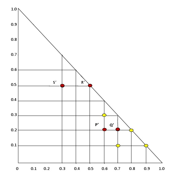
Where the maximum value of (10) rises the degree of possibility as well as the satisfaction level. This type is also known as Active focus point, because a decision maker take optimal solution according to this situation. Let us see the example which will help us to understand the formula (9). There are four state of nature \( y_1, y_2, y_3, y_4\). Possibility degree \(\lambda(\mathcal{M}(y), \mathcal{N}(y))\) is as:
\( \lambda(\mathcal{M}(y_1), \mathcal{N}(y_1))= (0.8,0.2), \lambda(\mathcal{M}(y_2), \mathcal{N}(y_2)) = (0.7,0.2), \lambda(\mathcal{M}(y_3), \mathcal{N}(y_3)) = (0.5,0.5), \lambda(\mathcal{M}(y_4), \mathcal{N}(y_4))\) \(= (0.7,0.1)\) and satisfaction level as: \( u((\mathcal{M}(y_1), \mathcal{N}(y_1)),b) = (0.6,0.2)\), \(u((\mathcal{M}(y_2), \mathcal{N}(y_2)),b) = (0.9,0.1)\), \(u((\mathcal{M}(y_3), \mathcal{N}(y_3)), b) = (0.6,0.3)\), \(u((\mathcal{M}(y_4), \mathcal{N}(y_4)),b) = (0.3,0.5)\) whose \([\lambda(\mathcal{M}(y), \mathcal{N}(y)), u(\mathcal{M}(y), \mathcal{N}(y),b)]\) points are: \( P = [\lambda(\mathcal{M}(y_1), \mathcal{N}(y_1)), u(\mathcal{M}(y_1), \mathcal{N}(y_1),b)] = [ (0.8,0.2), (0.6,0.2)]\) \( Q = [\lambda(\mathcal{M}(y_2), \mathcal{N}(y_2)), u(\mathcal{M}(y_2), \mathcal{N}(y_2),b)] = [ (0.7,0.2), (0.9,0.1)]\) \( R = [\lambda(\mathcal{M}(y_3), \mathcal{N}(y_3)), u(\mathcal{M}(y_3), \mathcal{N}(y_3),b)] = [(0.5,0.5), (0.6,0.3)]\) \( S = [\lambda(\mathcal{M}(y_4), \mathcal{N}(y_4)), u(\mathcal{M}(y_4), \mathcal{N}(y_4),b)] = [(0.7,0.1),(0.3,0.5)]\) \(\min[\lambda(\mathcal{M}(y), \mathcal{N}(y)), u(\mathcal{M}(y), \mathcal{N}(y),b)]\) represents to \(P’, Q’, R’, S’\) as: \( P’= \min [(0.8,0.2), (0.6,0.2)] = [(0.6,0.2), (0.6,0.2)]\) \( Q’= \min [(0.7,0.2), (0.9,0.1)] = [(0.7,0.2),(0.7,0.2)]\) \( R’= \min [(0.5,0.5), (0.6,0.3)] = [(0.5,0.5),(0.5,0.5)]\) \(S’= \min[(0.7,0.1),(0.3,0.5)] = [(0.3,0.5),(0.3,0.5)]\) and \(\max_{y\in S}\min [\lambda(\mathcal{M}(y), \mathcal{N}(y)), u(\mathcal{M}(y), \mathcal{N}(y),b)]\) is: \(\max \{[(0.6,0.2), (0.6,0.2)],[(0.7,0.2),(0.7,0.2)],[(0.5,0.5),(0.5,0.5)],\) \([(0.3,0.5)\), \((0.3,0.5)]\}\) \( = [(0.7,0.2),(0.7,0.2)]\) goes to \(Q’\). Thus, \(\arg\) \(\max_{y\in S}\min [\lambda(\mathcal{M}(y), \mathcal{N}(y)), u(\mathcal{M}(y), \mathcal{N}(y),b)]\) chooses \(y_2\). Figure 1. Explanation of (9).
In type 12th, the level of possibility is lowest as well as the level of satisfaction is greater.
3.2. Ideal (Optimal) Alternatives
In IOSDT problem we select various options (alternatives). These choices stimulate the decision maker at the time of the decision. And they totally depend on intuitionistic focus points. The categories related to alternatives are explained as under:
Let us show the method about the decision of the decision maker in intuitionistic one-shot decision with the help of example in next section.
4. Numerical Example
The set of alternatives is \(A = \{b_1, b_2, b_3\}\) and set of states is \(S = \{y_1, y_2, y_3\}\). The payoff on each state obtained for each alternative is listed in below. Let us suppose that the approximated possibility degrees and the satisfaction levels for alternatives for separately state are presented as:
Table 1. Possibility degrees.
Table 1. Possibility degrees.
\( \)
\(y_{1}\)
\(y_{2}\)
\(y_{3}\)
Possibilities
\((0.6,0.3)\)
\((0.75,0.2)\)
\((1,0)\)
Table 2. Satisfaction levels for each alternative.
\( \)
\(y_{1}\)
\(y_{2}\)
\(y_{3}\)
\(b_{1}\)
\((0.6,0.3)\)
\((1.0,0)\)
\((0.3,0.4)\)
\(b_{2}\)
\((0.75,0.2)\)
\((0.8,0.1)\)
\((0.8,0.1)\)
\(b_{3}\)
\((1,0)\)
\((0.2,0.2)\)
\((0.8,0.1)\)
Table 3. Payoffs for each alternative.
\( \)
\(y_{1}\)
\(y_{2}\)
\(y_{3}\)
\(b_{1}\)
\(600\)
\(1000\)
\(300\)
\(b_{2}\)
\(750\)
\(800\)
\(800\)
\(b_{3}\)
\(1000\)
\(200\)
\(800\)
For exemplary situation let us suppose \(\alpha\) = (0.7, 0.25) and \(\beta\) = (0.76, 0.15) so that the states are categorized in the following sets maintained by possibility degrees and satisfaction points;
i.e. \(Y^{\geq\alpha}=\{y_2, y_3\}\) (group continuing the high possibility degree), \(Y^{\leq\alpha}=\{y_1\}\) (group continuing the low possibility degree),
\(Y^{\geq\beta}(b_1)=\{y_2\}\) (group continuing the high satisfaction degree for alternative \(b_1\)), \(Y^{\leq\beta}(b_1)=\{y_1,y_3\}\) (group continuing the low satisfaction degree for alternative \(b_1\)), Similarly we can write for other alternatives as: \(Y^{\geq\beta}(b_2)=\{y_2, y_3\}\), \(Y^{\leq\beta}(b_2)=\{y_1\}\), \(Y^{\geq\beta}(b_3)=\{y_1, y_3\}\), \(Y^{\leq\beta}(b_3)=\{y_2\}\). According to all types which have been discussed in equations (1) to (12) are calculated and the final focus points according to certain order has been written in table 4. Let us write the detail of (9) to (12) as:
\(Y^{9}(b_1)= \max\{\min[(0.6,0.3), (0.6,0.3)], \min[(0.75,0.2), (1,0)]\), \(\min[(1,0)\), \((0.3\), \(0.4)]\}\) = \(\max\{[(0.6,0.3), (0.6,0.3)],
[(0.75,0.2), (0.75,0.2)]\), \([(0.3,0.4), (0.3,0.4)]\}\) = \([(0.75,0.2),(0.75,0.2)].\) Therefore, \([(0.75,0.2),(0.75,0.2)]\) corresponds to \(y_{2}.\)
\(Y^{10}(b_1)= \min\{\max[(0.6,0.3), (0.6,0.3)], \max[(0.75,0.2), (1,0)]\), \(\max[(1,0)\), \((0.3\), \(0.4)]\}\) = \(\min\{[(0.6,0.3), (0.6,0.3)],
[(1.0,0), (1.0,0)]\), \( [(1.0,0), (1.0,0)]\}\) = \([(0.6\), \(0.3)\), \((0.6,0.3)].\) Therefore, \([(0.6,0.3),(0.6,0.3)]\) corresponds to \(y_{1}\).
According to (11), \(Y^{11}(b_3)= \min\{\max[(0.3,0.6), (1,0)], \max[(0.2,0.75)\), \((0.2\), \(0.2)]\), \(\max[(0,1), (0.8,0.1)]\}\) = \(\min\{[(1.0,0), (1.0,0)],
[(0.2,0.2), (0.2,0.2)]\), \([(0.8\), \(0.1)\), \((0.8,0.1)]\}\) = \([(0.2,0.2),(0.2,0.2)].\) So, \(Y^{11}(b_3)\) = \(y_{2}.\)
According to (12), \(Y^{12}(b_3)= \min\{\max[(0.6,0.3), (0,1.0)], \max[(0.75,0.2)\), \((0.2\), \(0.2)]\), \(\max[(1,0), (0.1,0.8)]\}\) = \(\min\{[(0.6,0.3), (0.6,0.3)],[(0.75,0.2), (0.75,0.2)]\), \([(1.0,0)\), \((1.0,0)]\}\) = \([(0.6,0.3),(0.6,0.3)].\) Therefore, \([(0.6,0.3),(0.6,0.3)]\) corresponds to \(y_{1}\).
Hence, all the final focus points according to certain order has been listed in table 4.
Table 4. Focus points for each alternative.
\( \)
\(I\)
\(II\)
\(III\)
\(IV\)
\(V\)
\(VI\)
\(VII\)
\(VIII\)
\(IX\)
\(X\)
\(XI\)
\(XII\)
\(b_1\)
\(y_2\)
\(y_3\)
\(y_1\)
\(y_1\)
\(y_2\)
\(y_2\)
\(y_3\)
\(y_1\)
\(y_2\)
\(y_1\)
\(y_3\)
\(y_1\)
\(b_{2}\)
\(y_2,y_3\)
\(y_2,y_3\)
\(y_1\)
\(y_1\)
\(y_3\)
\(y_2\)
\(y_1\)
\(y_1\)
\(y_2\)
\(y_1\)
\(y_1\)
\(y_1\)
\(b_{3}\)
\(y_3\)
\(y_2\)
\(y_1\)
\(y_1\)
\(y_3\)
\(y_1\)
\(y_2\)
\(y_2\)
\(y_3\)
\(y_2\)
\(y_2\)
\(y_1\)
Table 5. Payoffs for focus points.
\( \)
\(I\)
\(II\)
\(III\)
\(IV\)
\(V\)
\(VI\)
\(VII\)
\(VIII\)
\(IX\)
\(X\)
\(XI\)
\(XII\)
\(b_1\)
\(1000\)
\(300\)
\(600\)
\(600\)
\(1000\)
\(1000\)
\(300\)
\(600\)
\(1000\)
\(600\)
\(300\)
\(600\)
\(b_{2}\)
\(800\)
\(800\)
\(750\)
\(750\)
\(800\)
\(800\)
\(750\)
\(750\)
\(800\)
\(750\)
\(750\)
\(750\)
\(b_{3}\)
\(800\)
\(200\)
\(1000\)
\(1000\)
\(800\)
\(1000\)
\(200\)
\(200\)
\(800\)
\(200\)
\(200\)
\(1000\)
According (13) to (24), final ideal alternative would be \(b_1,\) because in the above table the maximum value is 1000, so the optimal alternative goes to \(b_1\), similarly the other optimal alternatives are: \( b_2, b_3, b_3, b_1, \{b_1,b_3\}, b_2, b_2, b_1, b_2, b_2, b_3\).
Intuitionistic focus points in which attitudes of a decision maker has been expressed would have been discussed in (1) to (12). Now we inspect the connection that exits between these intuitionistic focus points.
5. Characteristics of Focus Points
The twelve types of focus points have been discussed in which shows the attitudes of decision maker about satisfaction and possibility. The relationship between the kinds of intuitionistic decision points are:
Theorem 5.1.
If \(Y^{1}_{\alpha}\),…, \(Y^{5}_{\beta}\),…, \(Y^{12}(b)\) represents the intuitionistic focus points, \(b\) is optimal alternative and \(\lambda\Big(\mathcal{M}(y), \mathcal{N}(y)\Big)\) is a possibility distribution where \(u\Big(\mathcal{M}(y), \mathcal{N}(y),b\Big)\) is the satisfaction function, then i. According to (1), (5) and (9)
where \(\alpha\) is fulfill (26) and is equal to (9). This implies that \(u\Big(\mathcal{M}(y^{‘}), \mathcal{N}(y^{‘}),b\Big)\geq\beta\), according to (33), \(\lambda\Big(\mathcal{M}(y^{‘}), \mathcal{N}(y^{‘})\Big)\) \(\geq\) \(\alpha\), it is clear that \( \min \Big[\lambda\Big(\mathcal{M}(y^{‘}), \mathcal{N}(y^{‘})\Big), u\Big(\mathcal{M}(y^{‘}), \mathcal{N}(y^{‘}),b\Big)\Big] \geq \alpha=\beta\), but we have \( \min \Big[\lambda\Big(\mathcal{M}(y^{‘}), \mathcal{N}(y^{‘})\Big), u\Big(\mathcal{M}(y^{‘}), \mathcal{N}(y^{‘}),b\Big)\Big] \leq \alpha=\beta.\) This implies that
The equation (34) and (35) show the way to \( Y^{1}_{\alpha}(b)\subseteq Y^{9}(b)\). In this manner, other case will be done. Hence (26) satisfied, and (28), (30) and (32) could also be proved.
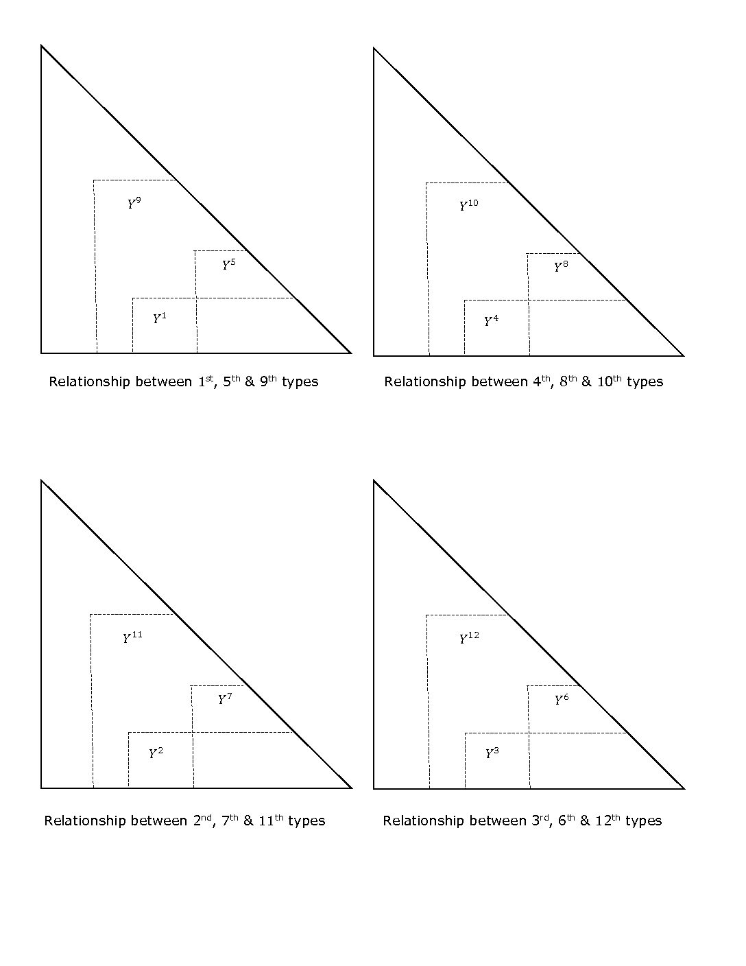
5.1. Graphical View Between Relationship of Types
Figure 2. Relationship between types.
The explanation of above theorem shows that the first type or the fifth type of decision points are the part of ninth type of decision point because the level of possibility and satisfaction in first type as well as in fifth type is high and the greatest respectively whereas in the ninth type the level of possibility and satisfaction is the greatest. Moreover, the union of fourth and eighth types is a subset of tenth type because the level of possibility and satisfaction in the 4th and 8th type is less and lesser respectively, whereas the level of possibility and satisfaction in tenth type is the lowest. The second and seventh types are mentioned in the eleventh types because the level of possibility and satisfaction is high and the lowest respectively in the eleventh type whereas the level of possibility and satisfaction in the second type is high and the lowest respectively. In the seventh type, the level of possibility and satisfaction is the highest and the lowest, respectively. The twelfth type of decision point holds third and sixth types. Because, the third type contains low possibility and the highest satisfaction, the sixth type contains lesser possibility and greater satisfaction and the twelfth type lesser possibility and greatest satisfaction level.
6. Conclusion
In this article, we discussed one-shot decision theory by using intuitionistic fuzzy sets because IFS is highly fruitful in expounding uncertain situations which we face in decision theory, and it is near the human mind set. OSD theory is a fundamental theory which highlights the human behavior. Intuitionistic one-shot decision is exemplary condition where a person has simply unique opportunity for judgement. We have reexamined the idea of IFS and suggested the applications which are relevant to intuitionistic one-shot decision method.
Various ideal points have been defined and they are entirely dependent upon the twelve kinds of focus points. The suggested decision patterns give us the ideal points as well as the true picture of the description which leads to such type of decision. As various focus points show the behavior of a person while the suggested decision patterns can give us effective information to comprehend the behavior of a person. The suggested intuitionistic fuzzy set theory can prove an effective tool for the analysis of one shot decision problem which are totally related with trade and economics.
In conclusion, one-shot decision problems e.g. in the introduction of new products study and progress and global dispute solution can be discussed.
In one-shot decision problems, a person gets only one chance for a decision. Therefore, the person has no opportunity to change the decision taken. Hence, we can say that IFS has a remarkable effect influence on the attitude of a person.
Competing Interests
The authors do not have any competing interests in the manuscript.
Acknowledgments
The author would like to thank the editor and the anonymous referee for their helpful comments.
References
Savage Leonard, J. (1954). The foundations of statistics. NY, John Wiley, 188-190. [Google Scholor]
George, J. K., & Tina, A. F. (1988). Fuzzy Sets Uncertainty and Information. Editorial Prentice Hall. [Google Scholor]
Knight, F. H. (1921). The meaning of risk and uncertainty. F. Knight. Risk, Uncertainty, and Profit. Boston: Houghton Mifflin Co, 210-235. [Google Scholor]
Guo, P. (2011). One-shot decision theory. IEEE Transactions on Systems, Man, and Cybernetics-Part A: Systems and Humans, 41(5), 917-926. [Google Scholor]
Baillon, A. (2008). Eliciting subjective probabilities through exchangeable events: An advantage and a limitation. Decision Analysis, 5(2), 76-87. [Google Scholor]
Zadeh, L. A. (1999). Fuzzy sets as a basis for a theory of possibility. Fuzzy sets and systems, 100(1), 9-34. [Google Scholor]
Dubois, D., Prade, H., & Sabbadin, R. (2001). Decision-theoretic foundations of qualitative possibility theory. European Journal of Operational Research, 128(3), 459-478. [Google Scholor]
Yager, R. R. (1979). Possibilistic decisionmaking. IEEE Transactions on Systems Man and Cybernetics, 9(7), 388-392.
Giang, P. H., & Shenoy, P. P. (2005). Two axiomatic approaches to decision making using possibility theory. European journal of operational research, 162(2), 450-467. [Google Scholor]
Bellman, R. E., & Zadeh, L. A. (1970). Decision-making in a fuzzy environment. Management science, 17(4), 141-164.[Google Scholor]
Bell, D. E. (1983). Risk premiums for decision regret. Management Science, 29(10), 1156-1166. [Google Scholor]
Atanassov, K. T. (1994). Operators over interval valued intuitionistic fuzzy sets. Fuzzy sets and systems, 64(2), 159-174. [Google Scholor]
Atanassov, K. T. (1999). Intuitionistic fuzzy sets. In Intuitionistic fuzzy sets (pp. 1-137). Physica, Heidelberg.[Google Scholor]
Atanassov, K. T. (1986). Intuitionistic fuzzy sets. Fuzzy sets and Systems, 20(1), 87-96. [Google Scholor]
Beg, I., & Rashid, T. (2014). Multi-criteria trapezoidal valued intuitionistic fuzzy decision making with Choquet integral based TOPSIS. Opsearch, 51(1), 98-129. [Google Scholor]
Szmidt, E., & Kacprzyk, J. (1997). On measuring distances between intuitionistic fuzzy sets. Notes on Intutiontisitic Fuzzy Sets, 3(4), 1-3. [Google Scholor]
Szmidt, E., & Kacprzyk, J. (2000). Distances between intuitionistic fuzzy sets. Fuzzy sets and systems, 114(3), 505-518.[Google Scholor]
Wang, W., & Xin, X. (2005). Distance measure between intuitionistic fuzzy sets. Pattern Recognition Letters, 26(13), 2063-2069.[Google Scholor]
Guo, P. (2010). Private real estate investment analysis within one-shot decision framework. International Real Estate Review, 13(3), 238-260. [Google Scholor]