This work is concerned with a comparative study of performances of meshfree (radial basis functions) and mesh-based (finite difference) schemes in terms of their accuracy and computational efficiency while solving multi-dimensional initial-boundary value problems governed by a nonlinear time-dependent reaction-diffusion Brusselator system. For computing the approximate solution of the Brusselator system, we use linearly implicit Crank-Nicolson (LICN) scheme, Peaceman-Rachford alternating direction implicit (ADI) scheme and exponential time differencing locally one dimensional (ETD-LOD) scheme as mesh-based schemes and multiquadric radial basis function (MQRBF) as a meshfree scheme. A few numerical results are reported.
Keywords: Brusselator systems, locally one dimensional, exponential time differencing, radial basis function collocation scheme, alternating direction implicit scheme.
1. Introduction
Reaction-diffusion systems arise frequently in the study of chemical and biological phenomena and are typically modeled by time-dependent partial differential
equations (PDEs) exhibiting oscillations. The dynamics of reaction-diffusion systems have been the subject of intense research activities over the past
few decades due to its ability to demonstrate very complex dynamic behavior such as periodic solution and chaos [1, 2, 3, 4]. It was argued in [5] that it is necessary to consider at least a cubic nonlinearity in the rate equations which originate from the model which was later referred as trimolecular model or Brusselator. The reaction-diffusion Brusselator system contains a pair of input chemicals which intermediate with two reactants to create two output (product)
chemicals of which concentrations are controlled under given conditions. The reaction scheme in Brusselator system contains an autocatlytic reaction as well as
trimolecular reaction step which occurs in the formation of ozone by atomic oxygen via a triple collusion. It also arises in the modeling of certain chemicals’
reaction-diffusion process such as enzymatic reactions, and in plasma and laser physics in multiple coupling between modes [6].
In many autocatlytic systems, complex dynamics have been observed, including multiple steady-states and periodic orbits which make Brusselator system so important
in the study of reaction-diffusion systems. But solving such systems analytically is either very challenging or next to impossible. That is why,
the reaction-diffusion Brusselator system is of interest from the numerical point of view.
Few researchers have proposed different approaches for approximating the solutions of one- and two-dimensional Brusselator systems. Adomian [6] used a decomposition method which was further modified by Wazwaz [7] for approximate solution of the reaction-diffusion Brusselator model. Among standard differencing schemes (mesh-based) developed for Brusselator systems, the numerical scheme (second order accurate in space and time) proposed by Twizell
et al.[8] is worth mentioning. Another robust and computationally economic scheme, known as Gauss-Seidel like implicit finite-difference scheme was proposed in [9] for solving the resulting PDEs from a coupled Brusselator model. This scheme not only provides comparable accuracy with the classical Runge-Kutta method, it is also unconditionally convergent. Later, standard and exponential time differencing (ETD) Crank-Nicolson (CN) methods were employed to solve the resulting initial-value problem from 1-D Brusselator system in [10]. To seek approximate solution of 2-D Brusselator system, a dual-reciprocity boundary element method was adopted in [11].
The finite difference method (FDM) uses local approximations to the differential operator and the boundary conditions by generating stencils of nodal values
that couple neighboring nodal values. In this sense, FDM differs from methods, such as Boundary Element method, which does not generate local stencils.
Basically, mesh-based methods like FDM require that the nodes of the stencils to be situated on some kind of
structured grid (or collection of structured grids), which severely limits their geometric flexibilities. This necessitates the development of meshfree approximating
schemes [12] e.g., collocation methods which need no mesh generation and usually allow numerous approaches to solve PDEs. Some of its favorable properties
which have contributed to its ever-increasing popularity among the scientific community are as follow:
ease to construct in any number of dimensions;
meshfree nature requiring only an arbitrary set of nodes to compute an approximate solution unlike the generation of full mesh needed, for instance, in FDM;
applicability to the irregular shape domain problem; and finally
capability to produce smooth approximations not only for the unknown
function but also for its derivatives. Known meshfree techniques for numerical simulation of 2-D Brusselator system are the radial basis
function (RBF) collocation method [1]iah}, and the method of lines (MOL) implemented as a meshfree method based on
spatial trial spaces spanned by the Newton basis functions [1]mms}.
In this work, multiquadric (MQ) RBF is used as meshfree scheme and linearly implicit Crank-Nicolson (LICN),
Peaceman-Rachford Alternative Direct Implicit (ADI), ETD locally one dimensional (ETD-LOD), and ETD-CN schemes
are used as mesh-based schemes to numerically simulate the 1-D and 2-D Brusselator systems.
2. Posing the problem
Let us consider the following initial-boundary value problems governed by the nonlinear time-dependent system of PDEs in order to implement mesh-based and
meshfree methods mentioned above:
2.1. Test problem 1
The Brusselator 1-D model in one spatial variable describing a chemical reaction with two constituents is given by the following system
of PDEs [10]
In Equation 4, \(a\) and \(b\) are concentrations of the two input reactants. Since the reactants \(A\) and \(B\) are assumed to be in such large access
so that their concentrations \(a\) and \(b\) do not change with time, therefore, considered as constants. Furthermore,
\(u\) and \(v\) represent dimensionless concentrations of two intermediate reactants and \(\mu\) is the constant diffusion coefficient.
3. Numerics
3.1. Mesh-based (finite difference) methods
3.1.1 Derivation of implicit Crank-Nicolson method for test problem 1
In order to implement linearly implicit Crank-Nicolson (LICN) to Test Problem 1, we discretized the domain \(\Omega\) with uniform grid of step size
\(h\) with \(h=1/(N-1)\), where \(N\) is the total number of grid points and partitioned time domain with time step \(k\). Let \(U_{i,j}\) and \(V_{i,j}\) denote the finite
difference approximations of \(u_{i,j}=u(ih,jk)\) and \(v_{i,j}=v(ih,jk)\) respectively. Now, we replaced \(u_{xx}\) with the mean of its finite-difference approximations i.e.,
\[u_{xx}\approx\frac {u_{i+1}^{j}-2u_{i}^j+u_{i-1}^j}{h^2}\]
with leading error of \(O(h^2)\) at the \((j)^{th}\) and \((j+1)^{th}\) time-levels as shown in the Figure 1.
Figure 1. Stencil for Linearly Implicit Crank-Nicolson (LICN) scheme.
Also, \(u_{t}\) being its forward difference approximation i.e., \(u_{t}\approx \dfrac{u_{i,j+1}-u_{i,j}}{k}\) with a leading error of \(O(k)\), we get:
which can be solved either by direct or indirect (iterative) methods for \(U_{i-1}^{j+1}\), \(U_i^{j+1}\), and \(U_{i+1}^{j+1}\) for \(i=2, 3…, N-1\).
Here, the system can be solved by using \(LU\) decomposition algorithm to attain the concentration profile of \(u\) of the Brusselator system
for successive time iterations. Similarly, the second equation of the above system can be solved for \(V_{i-1}^{j+1}, V_i^{j+1}\), and \(V_{i+1}^{j+1}\) for \(i=2, 3…, N-1\).
3.1.2 Construction of Peaceman-Rachford ADI scheme for test problem 2
The ADI is a predictor-corrector scheme, where part of the difference operator is implicit in the initial (predictor) step and another part is
implicit in the final (corrector) step. In Peaceman-Rachford, the predictor step consists of solving Test Problem 2 for a time step \(\frac {k}{2}\) using implicit
Euler method for the \(x\) derivative terms and the explicit Euler method for the \(y\) derivative terms i.e.,
The corrector step completes the solution process for a time step by using explicit Euler method for \(x\) derivative terms and the implicit Euler method for \(y\)
derivative terms, thus
where
\begin{equation*}
\textbf{U}^{n}=\left[\begin{array}{c}
U_{2,j}^{n}\\
U_{3,j}^{n}\\
\vdots\\
U_{N-1,j}^{n}\end{array}\right],
B^{n+\frac{1}{2}}=\left[\begin{array}{c}
U_{1,j}^{n+\frac{1}{2}}\\
\vdots\\
U_{N,j}^{n+\frac{1}{2}}
\end{array}
\right],
C^{n+1}=\left[\begin{array}{c}
U_{i,1}^{n+1}\\
\vdots\\
U_{i,N}^{n+1}
\end{array}
\right],
\end{equation*}
\(A_x = A_y =A\) as in Equation (9) and \(F(u,v,t)=u^2v-(b+1)u+a\). The system (14) can be efficiently solved by applying the LU decomposition
algorithm outside of the timing loop because the matrices \(A_x\) and \(A_y\) remain constant during the time iteration. Similarly, the second equations of
systems (12) and (13) can also be solved for \(V\) with the LU decomposition algorithm. This scheme is second order accurate both in time and
space and unconditionally stable and has restriction on time step such that \(k< 2h/\pi\) (approximately) to avoid oscillation where the discontinuity exist [15].
3.1.3 Derivation of ETD-LOD scheme for test problem 2
In order to derive ETD-LOD scheme for Test Problem 2, we introduce a uniform grid of spacing \(h\times h\) on domain \(\Omega\) with \(h=1/(N-1)\), where \(N\)
is the total number grid points along each direction \(x\) and \(y\). This allows the replacement of second order derivatives in Test Problem 2 by, for instance,
the central difference operator,
where \(\delta_x^2u(x,t)=u(x+h,t)-2u(x,t)+u(x-h,t)\), \ and \ \(\delta_y^2u(x,t)=v(x+h,t)-2v(x,t)+v(x-h,t)\).
Also, \(f(u,v,t)=u^{2}v-(b+1)u+a\) \ and \ \(g(u,v,t)=-u^{2}v+bu\).
Now, applying Equations (15) and (16) to all interior mesh points, we obtain a system of ordinary differential equations:
where \(\textbf{U}=\left[U_2,U_3,\cdots,U_{N-1}\right]\) is a vector of approximation to \(\textbf{u}=\left[u_2,u_3,\cdots,u_{N-1}\right]\).
Here \(A=A_1+A_2\), and though in general \(A_1\times A_2\neq A_2\times A_1\), here their multiplication is commutative due to the same diffusion coefficients involved with
second order derivatives in \(x\) and \(y\) and equal spatial step size length used along both the axes. In fact, \(A_1=A_2\) and
\begin{equation*}
\label{eq:gibson}
A_1=\frac{1}{h^{2}}\left[\begin{array}{cccccc} 2&-1&\cdots&0&0&0\\
-1&2&-1&\cdots&0&0\\ 0&-1&2&-1&\cdots&0\\
\vdots&\vdots&\ddots&\vdots&\vdots&\vdots\\
0&0&\cdots&-1&2&-1\\ 0&0&\cdots&0&-1&2\end{array}\right]
\end{equation*}
After solving Equation (17), formally we arrive at the following recurrence formula for the exact solution [10]:
Let the numerical approximation to \(\textbf{U}(t_n)\) and \(F(\textbf{U}_n\), \(\textbf{V}_n,t_n)\) be denoted by \(\textbf{U}_n\) and \(F_n\) respectively.
The simplest approximation to the integral is obtained by assuming \(F\) to be constant between \(t=t_n\) and \(t=t_{n+1}\) i.e., \(F=F_n+O(k)\) which makes it first order
accurate and subsequently yields
Now, we can compute (22) efficiently by using the Pade approximation \(R_{0,1}(kA)\) to approximate \(\exp(-kA_1)\) and \(\exp(-kA_2)\) in (23) which yields
where \(R_{0,1}(kA)=(I+kA)^{-1}\) and \(\textbf{U}^*\) is an intermediate vector.
Similarly, we can get the same expression for (18) as well. It is well-known that this two-step procedure is first-order accurate in time which also has the
advantage of being easily solved, when the components of second step of (24) are reordered. In particular, if the second order derivatives in Test Problem 2
are replaced by central differences, \(A\) becomes an \(N^2\times N^2\) matrix with five nonzero bands. Instead of solving such a banded system,
we solve (24) by implementing sequence of tridiagonal matrix solvers [15]. This scheme is also unconditionally stable and free of oscillatory problem
unlike Peaceman-Rachford ADI scheme.
3.2. Meshfree (radial basis functions) scheme
3.2.1 Construction of Meshfree RBF scheme for test problem 1
In order to implement meshfree approach to Test Problem 1 to get the unknown functions \(u\) and \(v\), we discretize the time derivatives of the
1-D Brusselator system by applying first order forward difference formula and the space derivatives by using \(\theta -\)\!weighted \((0\leq \theta\leq {1})\)
scheme at two successive time levels \(n\) and \(n+1\) as below:
where \(U^n{(x)}\approx u(x,t^n)\), \(V^n{(x)}\approx v(x,t^n)\), and \(\alpha_j^n\), \(\beta_j^n\) are unknown coefficients. Also \(r_j=\Vert x-x_j\Vert\), where
\(\Vert\cdot\Vert\) denotes the euclidean norm. The points \(x_j\) are the center points for \(j=1,2,\dots, N\), and lastly, \(\phi(r_j)\) are the RBFs.
In this work, for both Test Problems, we have used the multiquadric RBF, \(\phi(r)=\sqrt{r^2+c^2}\), where \(c\) is a positive shape parameter.
The aim is to determine the unknown coefficients in Equations (28) and (29) by the collocation method. Hence,
for each collocation point \(x_i,i=1,2,\dots, N\), Equations (28) and (29) can be expressed as
It should be noted that \(N = N_i+N_b\), where \(N_i\) is the number of interior points and \(N_b\) is the number of boundary points. The system of Equations (30) and
(31) can be expressed in matrix notation as
where
\begin{equation*}
\textbf{M}^n=\left[\begin{array}{c}
\textbf{U}^n\\
\textbf{V}^n\\
\end{array}\right],
\textbf{U}^n=\left[U_{1}^n,U_{2}^n,\dots,U_{N}^n\right]^{\prime}, \textbf{V}^n=\left[V_{1}^n,V_{2}^n,\dots,V_{N}^n\right]^{\prime},
\end{equation*}
\begin{equation*}
%\label{eq:gibson}
\textbf{B}=\left[\begin{array}{cc} \phi& \textbf{0}\\
\textbf{0}&\phi\end{array}\right],
\phi=\left[\begin{array}{c}
\phi_i\\
\phi_b\\
\end{array}\right],
\phi_i=\begin{array}{c}
(\phi(r_{i,j}))_{N_i\times N},i=1,\dots,N_i;j=1,2,\dots,N,
\end{array}
\end{equation*}
\begin{equation*}
\phi_b=\begin{array}{c}
\phi(r_{i,j})_{N_b\times N},i=N_{i}+1,\dots,N;j=1,2,\dots,N
\end{array},
\gamma^n=\left[\begin{array}{c}
\alpha^n\\
\beta^n\\
\end{array}\right],
\end{equation*}
\begin{equation*}
\alpha^{n}= \left[\alpha_{1}^n,\alpha_{2}^n,\dots,\alpha_{N}^n\right]^{\prime},\beta_n=\left[\beta_{1}^n,\beta_{2}^n,\dots,\beta_{N}^n\right]^{\prime}.
\end{equation*}
Plugging Equations (28) and (29) in to the system (27), we arrive at the following matrix form for Test Problem 1:
where
\begin{equation*}
%\label{eq:gibson}
\textbf{A}=\left[\begin{array}{cc}
2\textbf{U}^{n}\textbf{V}^{n}\circ\phi_i-(b+1)\phi_i+\mu \textbf{D}_1&(\textbf{U}^n)^2\circ\phi_i\\
b\phi_i- 2\textbf{U}^n\textbf{V}^n\circ\phi_i&\mu \textbf{D}_1-(\textbf{U}^n)^2\circ\phi_i\end{array}\right],
\end{equation*}
\begin{equation*}
%\label{eq:gibson}
\textbf{C}=\left[\begin{array}{cc}
-(b+1)\phi_i+\mu\textbf{D}_1&\textbf{0}\\
b\phi_i&\mu \textbf{D}_1\end{array}\right],
\textbf{D}=\left[\begin{array}{cc}
\textbf{0}&(\textbf{U}^n)^2\circ\phi_i\\
\textbf{0}&-(\textbf{U}^n)^2\circ\phi_i\end{array}\right],
\end{equation*}
\begin{equation*}
%\label{eq:gibson}
\textbf{P}^{n+1}=\left[\begin{array}{c}
\textbf{F}^{(n+1)}\\
\textbf{G}^{(n+1)}\\
\end{array}\right],\\
\end{equation*}
\begin{equation*}
\textbf{F}^{n+1}=\left[\begin{array}{c}
ak,ak,\cdots,ak,ak+f(x_{N_i+1},t^{n+1}),\cdots,ak+f(x_{N_i+1},t^{n+1})
\end{array}\right]^{\prime},
\end{equation*}
\begin{equation*}
\textbf{G}^{n+1}=\left[\begin{array}{c}
0,0,\cdots,0,g(x_{N_i+1},t^{n+1}),\cdots,g(x_{N_i+1},t^{n+1})
\end{array}\right]^{\prime},
\end{equation*}
\begin{equation*}
\textbf{D}_1=\begin{array}{c}
\left(\dfrac{\partial^2 \phi(r_{i,j})}{\partial x_{i}^2}\right)_{N_i\times N},i=1,2,\dots,N_i,j=1,2,\dots, N,
\end{array}
\end{equation*}
\(f(x,t)=1\) and \(g(x,t)=3\). The symbol \(\circ\) means the multiplication of \(i\)-th component of the vector \(\textbf{U}^n\) to every element of the \(i\)-th row
of the matrix \(\phi_i\).
To get \(2N\) unknown coefficients \(\alpha_j\) and \(\beta_j, j=1,2,\dots, N\) from the dense system (33), we solved it by using Gaussian elimination method.
The shape parameter \(c\) plays vital role to obtain an accurate solution, so it is imperative to evaluate the value of \(c\) numerically for each problem.
3.2.2. Construction of Meshfree RBF method for test problem 2
Implementing the same procedure as depicted in construction of meshfree RBF scheme for Test Problem 1, and just replacing\ \(r_{ij}=\Vert (x_i,y_i)-(x_j,y_j)\Vert\),
\(\phi(r_{ij})=\sqrt{r_{ij}^2+c^2}\) and \(\textbf{D}_1=\left(\textbf{C}_1+\textbf{C}_2\right)\)\ where
\begin{equation*}
\textbf{C}_1=\begin{array}{c}
\left(\frac{\partial^2 \phi(r_{i,j})}{\partial x_{i}^2}\right)_{N_i\times N},i=1,2,\dots,N_i, \quad j=1,2,\dots,N,
\end{array}
\end{equation*}
and
\begin{equation*}
\textbf{C}_2=\begin{array}{c}
\left(\frac{\partial^2 \phi(r_{i,j})}{\partial y_{i}^2}\right)_{N_i\times N},i=1,2,\dots,N_i, \quad j=1,2,\dots,N,
\end{array}
\end{equation*}
we can obtain similar expressions as in \eqref{eq:2:29} for Test Problem 2. Then, it can be solved by Gaussian
elimination method for \(2N\) unknown coefficients \(\alpha_j\) and \(\beta_j, j=1,2,\dots, N\).
4. Numerical results and discussions
In this section, we present the results of numerical schemes, namely meshfree (MQRBF) and mesh-based (finite difference)
outlined in the previous section for Test Problems 1 and 2, in order to carry out a comparative analysis of these schemes in terms of their accuracy,
rate of convergence and execution time. The accuracy of these schemes for both Test Problems is measured in terms of \(l_2\) norm error and
the temporal rate of convergence of schemes is calculated by using the following formula:
where \(e_{k}=\|u-u_{k}\|\), \(e_{\frac{k}{2}}=\|u-u_{\frac{k}{2}}\|\), \(u\) is an exact solution, \(u_{k}\) and \(u_{\frac{k}{2}}\)
are the numerical solutions at the time steps size \(k\) and \((k/2)\), respectively. The execution time is the CPU
time in seconds used by the schemes to get the solution of Test Problems.
Numerical solution of Test Problem 1 was computed by using the LICN, MQRBF and ETD-CN [1]kkw}
schemes at the final time \(t=10\). The \(l_2\) norm errors of these schemes were calculated by comparing their results with a reference solution obtained by employing the
implicit Euler method on very fine grid.
For the empirical convergence analysis, we set \(h=0.0125\), and by repeatedly halving the time step size \(k\) in each simulation, we calculate the \(l_2\) norm errors,
rates of convergence and CPU times which are presented in Table 1. As we can see from Table \ref{bruss1} that all three schemes are able to achieve the
expected order of convergence.
In terms of accuracy, MQRBF scheme with the weight parameter \(\theta=0.5\) outperforms other two schemes. But, in terms of computational efficiency,
we can observe that LICN and ETD-CN schemes take similar CPU time and perform more efficiently than MQRBF scheme.
For MQRBF scheme, the most accurate results are obtained corresponding to shape parameter \(c=0.12\) for \(N=81\).
Table 1. Comparison of the schemes LICN, ETD-CN and MQRBF for Test Problem 1 in terms of \(l_2\) norm error, rates of convergence,
and computational efficiency at \(t=10.0\) (only dimensionless concentration \(u\)).
LICN
ETD-CN [10]
MQRBF
k
\(l_{2}(u)\)
Order
CPU(s)
\(l_{2}(u)\)
Order
CPU(s)
\(l_{2}(u)\)
Order
CPU(s)
0.2
4.59E-02
–
0.0148
2.84E-02
–
0.0279
2.58E-03
–
0.2359
0.1
2.45E-02
0.9028
0.0297
6.45E-03
2.1392
0.0367
6.38E-04
2.0147
0.5882
0.05
1.27E-02
0.9472
0.0500
1.44E-03
2.1635
0.0480
1.59E-04
2.0013
1.2841
0.025
6.49E-03
0.9704
0.0750
3.62E-04
1.9892
0.0687
4.03E-05
1.9837
2.5373
Figure 2 exhibits the comparison of numerical solution obtained via LICN, ETD-CN, and MQRBF schemes with the analytical
solution for concentration profiles of \(u\) and \(v\) at \(t=10\). One can see from Figure 2, among three aforementioned
schemes, only ETD-CN and MQRBF solutions are in good agreement with the analytical solution.
Figure 2. Numerical solutions (obtained by the schemes LICN, ETD-CN, MQRBF) corresponding to \(h=0.0125\) \((N=81)\) and \(k=0.0125\) at \(t=10\) versus analytical solution.
In another set of experiments, we ran simulation on Test Problem 1 until \(t=10\) by using MQRBF to capture a spatio-temporal solution profile of the components \(u\) and \(v\) and shown in Figure 3.
Figure 3. Numerical solution obtained by MQRBF scheme for \(u\) and \(v\) corresponding to \((N=81)\) and \(k=0.0125\) until \(t=10\).
For Test Problem 2, the numerical computations are carried out using ETD-LOD, Peaceman-Rachford ADI and MQRBF schemes.
In order to verify whether the considered schemes demonstrate the expected convergence rates, a numerical test on Test Problem 2 was performed with various
values of \(k\) and fixed \(h=1/9\) (i.e., \(N=100\)) at \(t=2\). The computed results obtained from these schemes are displayed in Table \ref{bruss2}, where the empirical
convergence rates agree well with the expected rates of the schemes. Moreover, we observe that the scheme MQRBF outperforms the other two schemes in terms of
accuracy, but, it is computationally more expansive than ETD-LOD and Peaceman-Rachford ADI schemes. For MQRBF scheme, the most accurate results
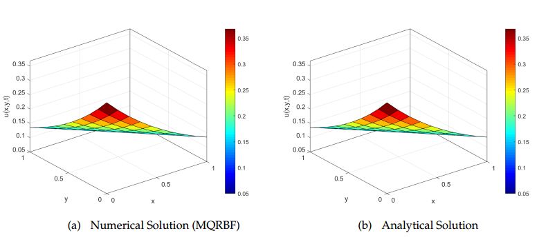
are obtained corresponding to shape parameter \(c=0.90\) for \(N=100\). Also the comparison of numerical approximations of \(u\), \(v\) via MQRBF scheme
and their corresponding analytical solutions are depicted through contour surface plots in Figure 4 and Figure 5 until \(t = 2\) for \(N = 100\).
Table 2. Comparison of the schemes ETD-LOD, Peaceman-Rachford ADI and MQRBF for Test Problem 2 in
terms of \(l_{2}\)−norm error, rates of convergence, and computational efficiency at \(t = 2.0\) (only for dimensionless
concentration \(u\)).
LICN
Peaceman-Rachford ADI
MQRBF
k
\(l_{2}(u)\)
Order
CPU(s)
\(l_{2}(u)\)
Order
CPU(s)
\(l_{2}(u)\)
Order
CPU(s)
0.2
8.01E-02
–
0.0085
1.19E-01
–
0.0451
5.73E-04
–
1.0106
0.1
3.98E-02
1.0071
0.0261
2.95E-02
2.020
0.0594
1.38E-04
2.0549
2.2406
0.05
1.99E-02
0.9987
0.0672
7.40E-03
1.9934
0.0867
3.30E-05
2.0623
4.6063
0.025
9.99E-03
0.9967
0.1382
1.93E-03
1.9377
0.1391
8.66E-06
1.9309
8.5403
Figure 4. Comparison between solution profiles of \(u\) with \(h=1/9\), \(k=0.01\) at \(t=2\).Figure 5. Comparison between solution profiles of \(v\) with \(h=1/9\), \(k=0.01\) at \(t=2\).
5. Conclusions
In this note, we presented a comparative study of mesh-based (e.g., LICN, ETD-CN, and Peaceman-Rachford ADI) and mesh free (MQRBF)
numerical schemes for solving 1-D and 2-D Brusselator systems. For both problems under consideration, the numerical results exhibited
that the meshfree scheme MQRBF provides more accurate approximations than other considered schemes in the note. In terms of computational efficiency,
MQRBF is more expansive than the mesh-based schemes used for the comparison. In the near future, we would like to investigate the
computational performances of RBF scheme and Fourier spectral schemes for solving three-dimensional
nonlinear reaction diffusion system.
Acknowledgments
The authors wish to express their profound gratitude to the reviewers for their useful comments on
the manuscript.
Author Contributions
All authors contributed equally to the writing of this paper. All authors read and approved the final manuscript.
Competing Interests
The author(s) do not have any competing interests in the manuscript.
References
Marek, M., & Schreiber, I. (1991). Chaotic Behavior of Deterministic Dissipative Systems. Cambridge University Press, New York. [Google Scholor]
Barkley, D., & Kevrekidis, I. G. (1994). A dynamical systems approach to spiral wave dynamics. Chaos: An Interdisciplinary Journal of Nonlinear Science, 4(3), 453-460. [Google Scholor]
Nicolis, G., & Prigogine, I. (1977). Self-organizations in Non-equilibrium Systems. Wiley-Interscience, New York. [Google Scholor]
Ault, S., & Holmgreen, E. (2003). Dynamics of the Brusselator. Unpublished manuscript, Department of Mathematics and Computer Science, Valdosta State
University, Georgia, USA. [Google Scholor]
Prigogine, I., & Lefever, R. (1968). Symmetries breaking instabilities in dissipative systems ii. Journal of Physical Chemistry, 48, 1695–1700. [Google Scholor]
Adomian, G. (1995). The diffusion-Brusselator equation. Computers & Mathematics with Applications, 29, 1–3. [Google Scholor]
Wazwaz, A. M. (2000). The decomposition method applied to systems of partial differential equations and to the reactions-diffusion Brusselator model. Applied Mathematics and Computation,110, 251–264. [Google Scholor]
Twizell, E. H., Gumel, A. B., & Cao, Q. (1999). A second-order scheme for the “Brusselator” reaction-diffusion system. Journal of Mathematical Chemistry , 26, 297–316. [Google Scholor]
Yu, P., & Gumel, A. B. (2001). Bifurcation and stability analysis for a coupled Brusselator model. Journal of Sound and Vibration, 244(5), 795–820. [Google Scholor]
Ang, W-T. (2003). The two-dimensional reaction–diffusion Brusselator system: a dual-reciprocity boundary element solution. Engineering Analysis with Boundary Elements, 27(9), 897–903.[Google Scholor]
Fasshauer, G. E. (2007). Meshfree Approximation Methods with Matlab. Vol. 6. World Scientific Pub. Co. Inc.[Google Scholor]
Siraj-ul-Islam, Ali, A., & Haq, S. (2010). A computational modeling of the behavior of the two-dimensional reaction-diffusion Brusselator system. Applied Mathematical Modelling, 34, 3896–3909. [Google Scholor]
Mohammadi, M., Mokhtari, R., & Schaback, R. (2014). A meshless method for solving the \textup{2D} Brusselator reaction-diffusion system. CMES – Computer Modeling in Engineering and Sciences, 101(2), 113–138. [Google Scholor]
Lawson, J. D., & Morris, J. LI. (1978). The extrapolation of first order methods for parabolic partial differential equations. SIAM Journal on Numerical Analysis ,15(6), 1212–1224.[Google Scholor]
Smith, G. D. (1996). Numerical Solution of Partial Differential Equations (3rd ed.). Oxford applied mathematics and computing science series. [Google Scholor]