1International Institute for Symmetry Analysis and Mathematical Modeling, Department of Mathematical Sciences, North-West University, Mafikeng Campus, Mmabatho 2735, South Africa.
2Department of Mathematics, Government College University, Faisalabad 38000, Pakistan.
The major purpose of this article is to discuss the oscillatory flow of an incompressible viscous Maxwell fluids (IVMF) between two infinite coaxial of circular pipes. In the case when time \(t=0\) the inner pipe is lying at rest where as at \(t>0\) the inner pipe of the annulus starts to oscillate along the common axis of the pipes. The analytical solutions of the problem are obtained via integral transformation technique which is beneficial for time dependent problems. Moreover, the derived solutions are given under the series form of the generalized \(G\) functions satisfying all the imposed auxiliary conditions whereas, the solutions for ordinary Maxwell and Newtonian fluids appear as the limiting case of the present obtained results. We include graphical comparison between Maxwell and Newtonian fluid, and we also explored the effects of different physical parameters on the fluid motion.
Unlike the Newtonian fluid, the model of non-Newtonian fluid is complex due to its non-linear behaviour. The non-Newtonian fluid are found in food industry, medical sciences, bio chemistry and engineering, therefore it is important to understand the non-Newtonian fluid models. There is no specific model that exactly describe the rheological behaviour of non-Newtonian fluids. Models, such as Maxwell, Oldroyd-B, second grade and Burgers’ are of great importance.
Lee and Finlayson [1] established the stability of Couette and plane Poiseuille flow of a Maxwell fluid. They used the Newton Raphson iteration method on the eigenvalues. Choi et al. [2] studied the two dimensional Maxwell’s fluid in porous channel. By considering the effects of viscoelasticity and inertia, the problem is solved in both way analytically and numerically. They also discussed its application on injection flow of Maxwell’s fluid. Karra et al. [3][2010]} studied the Maxwell’s model of viscoelastic fluid by assuming that the viscosity and relaxation parameters are depending on pressure. They also solved the boundary value problem using a generalized Maxwell’s and pressure dependent model. Vieru et al. [4] considered the infinite circular cylinder and determined the exact solutions of Maxwell fluid for oscillation (both longitudinal and torsional) with the help of the Laplace transformation. Time-periodic motion was discussed in the form of steady state solution that are free from initial conditions. The study of unsteady fractional Maxwell’s fluid between two circular domains have been done by Fetecau et al. [5]. Initially, they considered the fluid at rest position and after that they assumed that the fluid is moving due to the motion of inner cylinder. The motion in the fluid begin with the motion of inner cylinder and they find the results in the form of \(G\) and \(R\) functions.
Mathur et al. [6] obtained the exact solutions of viscoelastic fluid in pipe like domain with Maxwell model between annulus of the cylinders. The torsional stress (time dependent) on inner pipe producing motion in fluid where as outer pipe is moving with constant velocity. Mathur et al. [7] also obtained the exact solution of fractional Maxwell fluid moving between two coaxial infinite circular cylinders due to oscillation. Finite Hankel and Laplace transform has been used with boundary conditions i.e both the cylinders start to oscillate about their common axis. Akhtar et al. [8] find out the exact solutions of an incompressible generalized Maxwell’s fluid between circular cylinders by mean of rotation. They wrote their results in the form of generalized function by using Laplace and finite Hankel transformation.
Fetecau and Cornia [9] examined the flow behaviour of an Oldroyd-B fluid produced by instantly moving smooth plates. Accurate solutions for velocity field and its corresponding tangential tension are found by using the integral transform method, solutions for second grade and Maxwell fluids are also discussed. Bandelli [10] have carried out a research on the heated edges of the unsteady unidirectional flows of second grade fluids and derived the energy equation for second grade fluids. Also, they determined accurate results for different flows. Safdar et al. [11] derived the exact solutions for the flow model of generalized Burger’s fluid with in pipe like domain by using the similar integral transformation technique. They also obtained the numerical solutions for the same fluid and flow. An et al. [12] numerically studied the oscillatory flow between two cylinders with two different diameters. Finite element method is used to solve the Navier-Stokes equations. The interesting result is that the flow field between two cylinders is different from the single case, specially when diameters of cylinders are increasing. Similarly, many mathematicians applied fractional derivative approach and integral transformation technique on different fluid models [13, 14, 15].
2. Mathematical formation of the problem
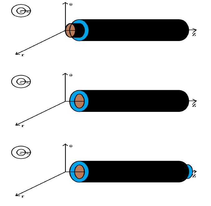
Let us consider an IVMF in an annulus of two pipes with radii \(R_{i}\) and \(R_{O}\) of inner and outer pipe respectively. Also, assuming that the outer pipe is fixed while inner pipe is oscillating. Imposing, the initial and boundary conditions as,
where
\begin{align*}
B_{1}(\varrho\varrho_{n})= J_{0}(\varrho\varrho_{n})Y_{0}(R_{i}\varrho_{n})-J_{0}(R_{i}\varrho_{n})Y_{0}(\varrho\varrho_{n})
\end{align*}
and \(\varrho_{n}\) are the positive roots of equation, also \(B_{1}(R_{O}\varrho_{n})=0\). Here \(J_{p}(.)\) and \(Y_{p}(.)\) are the Bessel functions of first and second kind of order \(p\). The Hankel transform of \(\overline{w}(\varrho,s)\) can be defined as
\begin{align*}
\overline{w}(\varrho_{n},s)=\int_{R_{i}}^{R_{O}}\varrho B_{1}(\varrho\varrho_{n})\overline{w}(\varrho,s)d\varrho,
\end{align*}
and its inverse Hankel transform is
\begin{align*}
\overline{w}(\varrho,s)= \frac{\pi^{2}}{2}\sum_{n=1}^{\infty}\frac{\varrho_{n}^{2}J_{1}^{2}(R_{O}\varrho_{n}) B_{1}(\varrho\varrho_{n})}{J_{1}^{2}(R_{i}\varrho_{n})-J_{1}^{2}(R_{O}\varrho_{n})}\overline{w}(\varrho_{n},s).
\end{align*}
Integrating by parts Equation (7) becomes as
Using the identity Equation (14) and applying the Laplace inverse transform, the final form of velocity field is
\begin{align*}
w(\varrho,t)= -\frac{(\mathfrak{A} Sin\Omega t)R_{i}(\varrho^{2}-R_{O}^{2})}{(R_{O}^{2}-R_{i}^{2})\varrho}+ \mathfrak{A} \pi \sum_{n=1}^{\infty}\frac{J_{0}^{2}(R_{O}\varrho_{n})B_{1}(\varrho\varrho_{n})}{J_{0}^{2}(R_{i}\varrho_{n})-J_{0}^{2}(R_{O}\varrho_{n})}\frac{1}{\rightthreetimes^{\beta}}\sum _{k=0}^{\infty}{\left(\frac{-\nu \varrho_{n}^{2}}{\rightthreetimes^{\beta}}\right)}^{k}
\end{align*}
\begin{align}\label{15}
\times\left[\int_{0}^{t}Sin\Omega(t-\tau)\mathrm{G}_{\beta,-k,k+1}\left(\frac{-1}{\rightthreetimes^{\beta}},t\right) dt+ \rightthreetimes^{\beta} \int_{0}^{t}Sin\Omega(t-\tau)\mathrm{G}_{\beta,\beta-k,k+1}\left(\frac{-1}{\rightthreetimes^{\beta}}, t \right)dt\right], %15
\end{align}
(15)
where \(\mathrm{G}_{a,\,b,\,c}(.\,,\,t)\) is the generalized function, as defined in [Equations (97) and (101)] [17]
Dividing the term \((1+\rightthreetimes^{\beta} s^{\beta})\) both sides and applying the inverse Laplace transform
\begin{eqnarray*}
\tau(\varrho,t)= \frac{\mu}{\rightthreetimes^{\beta}}\left[\frac{-2AR_{i}^{2}R_{O}^{2}}{(R_{O}^{2}-R_{i}^{2})\varrho^{2}}+\pi \mathfrak{A}\sum_{n=1}^{\infty}\frac{J_{1}(R_{O}\varrho_{n})[\varrho\varrho_{n}B_{0}(\varrho\varrho_{n})-2B_{1}(\varrho\varrho_{n})]}{\varrho[J_{1}^{2}(R_{i}\varrho_{n})-J_{1}^{2}(R_{O}\varrho_{n})]} \right]\times\int_{0}^{t} Sin\Omega(t-\tau)\mathrm{G}_{\beta,0,1}\left( \frac{-1}{\rightthreetimes^{\beta}}, t \right)dt
\end{eqnarray*}
where \(\mathrm{G}_{a,\,b,\,c}(.\,,\,t)\) is the generalized function.
3. Limiting Cases
3.1. Ordinary Maxwell fluid
Setting \(\beta\rightarrow1\) in Equations (15) and (19), we have the expression for ordinary Maxwell’s fluid i.e
\begin{align*}
w(\varrho,t)= -\frac{(\mathfrak{A} Sin\Omega t)R_{i}(\varrho^{2}-R_{O}^{2})}{(R_{O}^{2}-R_{i}^{2})\varrho}+ \mathfrak{A} \pi \sum_{n=1}^{\infty}\frac{J_{1}^{2}(R_{O}\varrho_{n})B_{1}(\varrho\varrho_{n})}{J_{1}^{2}(R_{i}\varrho_{n})-J_{1}^{2}(R_{O}\varrho_{n})}
\frac{1}{\rightthreetimes}\sum _{k=0}^{\infty}\left(\frac{-\nu \varrho_{n}^{2}}{\rightthreetimes}\right)^k
\end{align*}
and
\begin{eqnarray*}
\tau(\varrho,t)= \frac{\mu}{\rightthreetimes}\left[\frac{-2AR_{i}^{2}R_{O}^{2}}{(R_{O}^{2}-R_{i}^{2})\varrho^{2}}\int_{0}^{t} Sin\Omega(t-\tau)\mathrm{G}_{1,0,1}\left( \frac{-1}{\rightthreetimes}, t \right)dt+\pi \mathfrak{A}\sum_{n=1}^{\infty}\frac{J_{1}(R_{O}\varrho_{n})[\varrho\varrho_{n}B_{0}(\varrho\varrho_{n})-2B_{1}(\varrho\varrho_{n})]}
{\varrho[J_{1}^{2}(R_{i}\varrho_{n})-J_{1}^{2}(R_{O}\varrho_{n})]} \right]
\end{eqnarray*}
\begin{eqnarray}\label{21}
\times \frac{1}{\rightthreetimes}\sum_{k=0}^{\infty}\left(\frac{-\nu \varrho_{n}^{2}}{\rightthreetimes}\right)^{k}\left[\int_{0}^{t} Sin\Omega(t-\tau)\mathrm{G}_{1,-k,k+2}\left( \frac{-1}{\rightthreetimes}, t \right)dt+\mathfrak{\rightthreetimes}\int_{0}^{t} Sin\Omega(t-\tau)\mathrm{G}_{1,1-k,k+2}\left( \frac{-1}{\rightthreetimes}, t \right)dt\right]. %21
\end{eqnarray}
(21)
3.2. Newtonian fluid
By making \(\rightthreetimes^{\beta} \rightarrow 0\) in Equations (15) and (19) and using the following result
\begin{eqnarray*}
\lim_{\rightthreetimes^{\beta}\rightarrow 0}\frac{1}{\rightthreetimes^{k}}\mathrm{G}_{1,-k,k+1}(-\rightthreetimes^{-\beta}, t)= \frac{t^{k-1}}{\Gamma(k)},\,\,\, k< 0.
\end{eqnarray*}
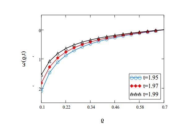
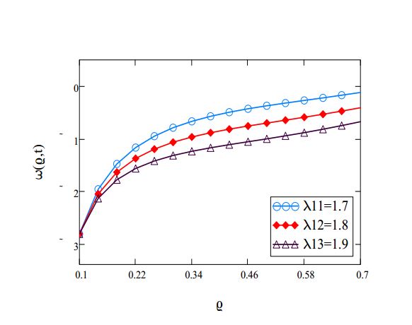
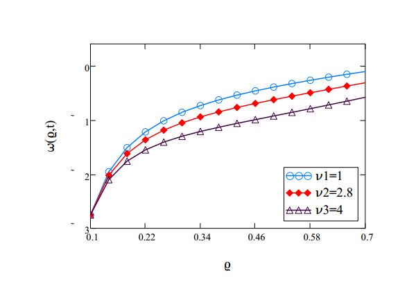
Figure 2.The influence of velocity \(w(\varrho,t)\) for \(R_{i}=0.1\), \(R_{o}=0.7\), \(\beta=0.85\), \(\rightthreetimes=2\), \(\mathfrak{A}=5\), \(\nu=0.45\) and \(\Omega=3\) with various values of \(time\).Figure 3. The influence of velocity \(w(\varrho,t)\) for \(R_{i}=0.1\), \(R_{o}=0.7\), \(\beta=0.85\), \(t=1.87\), \(\mathfrak{A}=5\), \(\nu=0.35\) and \(\Omega=2\) with various values of \(\rightthreetimes\).Figure 4. The influence of velocity \(w(\varrho,t)\) for \(R_{i}=0.1\), \(R_{o}=0.7\), \(t=1.90\), \(\rightthreetimes=2\), \(\mathfrak{A}=5\), \(\nu=0.45\) and \(\Omega=3\) with various values of \(\beta\).Figure 5. The influence of velocity \(w(\varrho,t)\) for \(R_{i}=0.1\), \(R_{o}=0.7\), \(\beta=0.85\), \(t=1.90\), \(\rightthreetimes=3\), \(\mathfrak{A}=5\) and \(\Omega=3\) with various values of \(\nu\).Figure 6. The influence of velocity \(w(\varrho,t)\) for \(R_{i}=0.1\), \(R_{o}=0.7\), \(\beta=0.85\), \(t=1.90\), \(\rightthreetimes=2\), \(\mathfrak{A}=5\), \(\nu=0.45\) and \(\Omega=3\) for comparison of Maxwell and Newtonian fluids.
5. Results and Discussion
The present paper, describe the oscillatory flow of an incompressible viscous Maxwell fluids passing through the infinite coaxial of circular pipes. The outer pipe is at rest and inner pipe is oscillating with respect to time. The time dependent results for velocity profile and shear stress are derived above. In this section, we discuss the nature of different fractional and physical parameters including in the results.
Figure 1 shows the behaviour of time parameter with respect to velocity. The parameter \(\varrho\in\{0.1,0.2,…,0.7\}\) and point to point value can also observed from the graph. Here, we take the fixed values of inner cylinder \(0.1\), outer cylinder \(0.7\), fractional parameter \(0.85\), relaxation parameter \(2\), constant \(\mathfrak{A}=5\), dynamic viscosity \(0.45\) and angular parameter \(\Omega=3\). Figure 2 depict the decreasing nature of relaxation parameter \(\rightthreetimes\) with respect to velocity. The influence of fractional variable \(\beta\) is increasing with the increase in velocity as in Figure 3. Dynamic viscosity \(\nu\) have decreasing behaviour with increase in the velocity parameter shown in Figure 4. All other involved parameters are remain fixed also for this graph given in the caption of Figure 4. Comparison of Newtonian and Maxwell fluids are given in Figure 5 which showa that the Maxwell fluid has more viscosity than the Newtonian fluid.
Author Contributions
All authors contributed equally to the writing of this paper. All authors read and approved the final manuscript.
Competing Interests
The author(s) do not have any competing interests in the manuscript.
References
Lee, K. C., & Finlayson, B. A. (1986). Stability of plane Poiseuille and Couette flow of a Maxwell fluid. Journal of non-newtonian fluid mechanics, 21(1), 65-78. [Google Scholor]
Choi, J. J., Rusak, Z., & Tichy, J. A. (1999). Maxwell fluid suction flow in a channel. Journal of non-newtonian fluid mechanics, 85(2-3), 165-187.[Google Scholor]
Karra, S., Prusa, V., & Rajagopal, K. R. (2011). On Maxwell fluids with relaxation time and viscosity depending on the pressure. International Journal of Non-Linear Mechanics, 46(6), 819-827.[Google Scholor]
Vieru, D., Akhtar, W., Fetecau, C., & Fetecau, C. (2007). Starting solutions for the oscillating motion of a Maxwell fluid in cylindrical domains. Meccanica, 42(6), 573-583. [Google Scholor]
Fetecau, C., Fetecau, C., Jamil, M., & Mahmood, A. (2011). RETRACTED ARTICLE: Flow of fractional Maxwell fluid between coaxial cylinders. Archive of Applied Mechanics, 81(8), 1153-1163.
[Google Scholor]
Khandelwal, K., & Mathur, V. (2015). Exact solutions for an unsteady flow of viscoelastic fluid in cylindrical domains using the fractional Maxwell model. International Journal of Applied and Computational Mathematics, 1(1), 143-156. [Google Scholor]
Mathur, V., & Khandelwal, K. (2017). Flow of Fractional Maxwell Fluid in Oscillating Pipe-Like Domains. International Journal of Applied and Computational Mathematics, 3(2), 841-858.[Google Scholor]
Akhtar, W., Siddique, I., & Sohail, A. (2011). Exact solutions for the rotational flow of a generalized Maxwell fluid between two circular cylinders. Communications in Nonlinear Science and Numerical Simulation, 16(7), 2788-2795. [Google Scholor]
Fetecau, C., & Fetecau, C. (2003). The first problem of Stokes for an Oldroyd-B fluid. International Journal of Non-Linear Mechanics, 38(10), 1539-1544.[Google Scholor]
Bandelli, R. (1995). Unsteady unidirectional flows of second grade fluids in domains with heated boundaries. International journal of non-linear mechanics, 30(3), 263-269.[Google Scholor]
Safdar, R., Imran, M., & Khalique, C. M. (2018). Time-dependent flow model of a generalized Burgers’ fluid with fractional derivatives through a cylindrical domain: An exact and numerical approach. Results in Physics, 9, 237-245.[Google Scholor]
An, H., Cheng, L., Zhao, M., & Dong, G. (2006, January). Numerical simulation of oscillatory flow around two circular cylinders of different diameters. In 25th International Conference on Offshore Mechanics and Arctic Engineering (pp. 35-43). American Society of Mechanical Engineers.[Google Scholor]
Friedrich, C. H. R. (1991). Relaxation and retardation functions of the Maxwell model with fractional derivatives. Rheologica Acta, 30(2), 151-158. [Google Scholor]
Awan, A. U., Imran, M., Athar, M., & Kamran, M. (2013). Exact analytical solutions for a longitudinal flow of a fractional Maxwell fluid between two coaxial cylinders. Journal of Mathematics (ISSN 1016-2526), 45, 9-23. [Google Scholor]
Fetecau, C., & Fetecau, C. (2004). Unsteady helical flows of a Maxwell fluid. Proceedings of the Romanian Academy Series A, 5(1), 13-19.[Google Scholor]
Ali, A., Tahir, M., Safdar, R., Awan, A. U., Imran, M., & Javaid, M. (2018). Magnetohydrodynamic Oscillating and Rotating Flows of Maxwell Electrically Conducting Fluids in a Porous Plane. Punjab University Journal of Mathematics, 50, 61-71.[Google Scholor]
Lorenzo, C. F., & Hartley, T. T. (1999). Generalized functions for the fractional calculus. NASA/TP—1999-209424/REV1[Google Scholor]