Flow of viscous fluid over an infinite plate with Caputo-Fabrizio derivatives

1. Introduction

The concept of fractional order derivatives is as old as for integer order derivatives. For the past three decades, this subject was limited only to mathematics. However, in the last few years, the concepts of fractional calculus were frequently applied to other disciplines. Recently, this subject has been extended in various directions such as fractional-order multipoles in electromagnetism, electrochemistry, tracer in fluid flows, model of neurons in biology, finance, signal processing, applied mathematics, bio engineering, viscoelasticity, fluid mechanics and fluid dynamics [1]. In fluid dynamics, the fractional derivative models are used widely for the study of viscoleastic materials such as polymers in the glass transition and glassy state [2]. Recently, it is increasingly seen as an efficient tool through which useful generalization of physical concept can be obtained. The most used fractional derivatives are the Riemann-Liouville fractional derivative and the Caputo fractional derivative [3, 4, 5, 6, 7]. It is known that, these operators exhibit difficulties in applications. For example, the Riemann-Liouvile derivative of a constant is not zero and, the Laplace transform of the Riemann-Liouville derivative contains terms without physical signification. The Caputo fractional derivative has eliminated these difficulties, but, the kernel of definition is a singular function. Caputo and Fabrizio have introduced recently, a new definition of the fractional derivatives with an exponential kernel without singularities [8]. The Caputo-Fabrizio temporal-fractional derivative is suitable to use the Laplace transform. The spatial representation of the Caputo-Fabrizio derivative is adequate to use the Fourier transform.

The aim of this report is to use the definition of Caputo-Fabrizio fractional derivative in order to obtain exact general solutions for the flow of an incompressible fractional viscous fluid over an infinite plate that is moving in its plane. The solutions that have been obtained are presented in simple forms and can be easily reduced to the similar solutions for ordinary fluids. Also compression of fractional and ordinary fluid are presented numerically and graphically. Rest of the paper is arranged as follows. The mathematical formulation of the problem is given in Section 2. Exact solutions via Laplace transform are established in Section 3 followed by some limiting cases in Section 4 and special cases in Section 5. Graphical results are portrayed in Section 6. This paper ends with some important conclusion in Section 7. Some important formulas used in this paper are presented in Appendix.

2. Mathematical formulation of the problem

We consider an incompressible viscous fluid occupying the space over an infinite plate which is situated in the \((x,z)-\)plane of the Cartesian coordinate system with the positive \(y-\)axis in the upward direction. Initially, both the fluid and the plate are at rest. At \(t=0^+\), the fluid is set in motion by the plate, which begins to move along the \(x\)-axis. The velocity of the plate is assumed to be of the form \(U_{0}f(t)\), where \(U_{0}>0\) is a constant and \(f(t)\) is a piecewise continuous function defined on \([0, \infty \left.\right)\) and \(f(0) = 0\). Furthermore, we suppose that the Laplace transform of the function \(f(t)\) exists. In the case of parallel flow along the \(x\)-axis, the velocity vector is \(V ={u(y,t),0,0}\) leads us to the following governing equations: where \(v\) is the kinematic viscosity, \(\tau(y,t) = S_{xy}{(y,t)}\) is the nonzero shear stress, \(\mu\) is the dynamic viscosity of the fluid. The adequate initial and boundary conditions are given by Introducing the following non-dimensional quantities to equations (1), (2) and (3);
\(t^* = \frac{t}{T}\); \(T>0\), \(y^*=\frac{y}{U_0 T}\), \(u^* = \frac{u}{U_0}\), \(\tau^* = \frac{\tau}{\rho U_0^2}\), \(f^*(t^*)= f(Tt^*)\),
and dropping out the '*' notation, we get the following non-dimensional problem: The non-dimensional initial and boundary conditions are where Re \(= \dfrac{U_0^2 T}{v}\) is the Reynolds number. In order to develop a model with time-fractional derivatives, we replace the first order time derivative with Caputo-Fabrizio time-fractional derivative of order \(\alpha \in {0,1}\). Thus, (4) is written as, where Caputo-Fabrizio time-fractional derivative [8] is defined as,

3. Calculation for velocity field

If we apply the Laplace transform to equation (9) and conditions (7), (8) and use the initial conditions, we get the following. where \(\overline{u}(y,q)\) and \(F(q)\) are the Laplace transform of \(u(y,t)\) and \(f(t)\) respectively, and '\(q\)' is the transform variable. The solution of the partial differential equation (11) by using conditions (12) and (13) is given as Similarly, (14) can be written in the equivalent form as, Applying the inverse Laplace transform and using convolution product, we obtain where \( f'(t)=L^{-1}\{qF(q)\}\) and \(\phi(y,t;a,b) = L^{-1}\{\Phi(y,q;a,b)\}\) is defined in Appendix (A1) and (A2).

4. Velocity field to ordinary viscous fluid case (\(\alpha=1\))

The velocity field, corresponding to the ordinary case of \(\alpha=1\), is obtained by using the properties of Caputo-Fabrizio fractional derivative. Consider the following. Using (10), we get, we obtain which gives the velocity field as follows.

5. Special Cases

In order to discuss the theoretical and practical value of general solutions and to certify their accuracy or to gain some physical insight for some motions with technical relevance, three special cases are considered in the following. Actually, these general solutions can provide the dimensionless velocity field corresponding to any motion problem of this type of fluids. \subsection{Plate moves with constant velocity: \(\{f(t) = H(t)\}\)} Let \(H(\cdot)\) be the Heaviside unit step function. Then, the dimensionless velocity field, representing the motion induced by an infinite plate that is moving in its plane, with a constant velocity is as follows. \begin{equation*} u(y,t) = \int_{0}^{t} \delta(t-s) \phi\{y,s; \text{ Re}\gamma,\alpha\gamma\}ds = \phi\{y,t; \text{ Re}\gamma,\alpha\gamma\}. \end{equation*} \subsection{Plate moves with oscillating velocity: \(\{f(t) = \sin(t)\}\)} The dimensionless velocity field, representing the solution corresponding to motions due to a plate that is oscillating in its plane, is given by, \begin{equation*} u(y,t) = \int_{0}^{t} \cos\{t-s\}\phi\{y,s; \text{ Re}\gamma,\alpha\gamma\}ds. \end{equation*} \subsection{Plate moves with exponential velocity: \(\{f(t) = H(t)\exp(at)\}\)} The dimensionless velocity field is \begin{equation*} u(y,t) = \phi(y,t; \text{ Re}\gamma,\alpha\gamma) + \psi(y,t; \text{ Re}\gamma,\alpha\gamma,c) \end{equation*} where \(\psi(y,t; a,b,c)\) is defined in Appendix (A3).

6. Numerical results and discussions

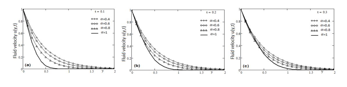
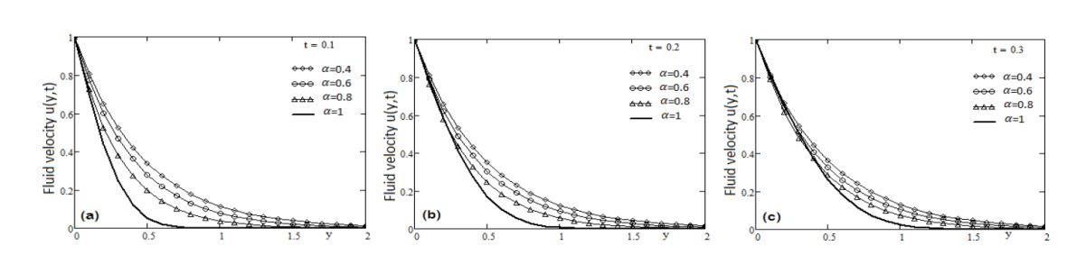
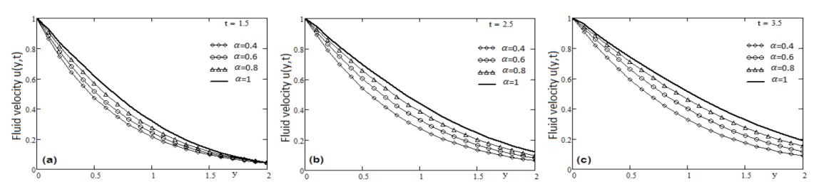
In order to obtain some information on the fluid flow parameters, we have made several numerical simulations using Mathcad software. Obtained results are presented in the Figures 1 - 3. All the parameters and profiles are dimensionless. For curves we consider the function \(f(t) = H(t)\). We are interested, first, to analyze the influence of the fractional parameter, \(\alpha\), on the dimensionless fluid flow velocity. Also, the influence of the Reynolds number, Re, on the fluid velocity were studied. The ordinary fluid, corresponding to the unit fractional parameter, is compared with few cases with the fractional parameter. The Figures 1 and 2 are plotted in order to discuss the influence of the fractional parameter \(\alpha\) on the fluid velocity. The curves corresponding to fluid velocity \(u(y,t)\), are sketched versus \(y\), for small and large values of time and of fractional parameter \(\alpha\), namely, \(\alpha \in \{0.4,0.6,0.8,1.0\}\). For Reynolds number, we used the value Re\( = 3\). The Figure 1 is plotted for small time \(t\). It is observed that by increasing values of the fractional parameter \(\alpha\), the fluid velocity decreases and by increasing the time \(t\), the difference between the fluid velocities decreases. Figure 2 is plotted for large time \(t\). It is observed that it has opposite behavior from Figure 1. The influence of Reynolds number on the fluid velocity is shown in Figure 3. For curves plotted in Figure 3, the fractional model corresponding to \(\alpha = 0.5\) was considered. It is observed from Figure 3 that, at small values of Reynolds number, the velocity is larger. It is also observed that for small and large values time \(t\), the behavior is same only by increasing the values of time \(t\), the difference between the velocities is significant.

7. Conclusions

We presented a model of Newtonian fluid with Caputo-Fabrizio fractional derivatives, over an infinite flat plate together with general boundary motion. Closed form exact general solutions of the fluid velocity are obtained by means of the Laplace transform. The following are observations:

1. It is observed that by increasing values of the fractional parameter, the fluid velocity decreases.
2. By increasing the time \(t\), the difference between the fluid velocities decreases.
3. At small values of Reynolds number, the velocity is larger.
4. It is also observed that for small and large values of time \(t\), the behavior is same only by increasing the values of time \(t\), the difference between the velocities is significant.

Appendix

\begin{equation}\tag{A1} \Phi(y,s;a,b) = \frac{1}{s}\exp\left\{-y\sqrt{\frac{as}{s+b}}\right\}.\end{equation} \begin{equation}\tag{A2}\phi(y,t; a,b) = L^{-1}(\Phi(y,s; a,b)) = 1 - \frac{2a}{\pi}\int_{0}^{\infty}\frac{\sin(yx)}{x\{a+x^2\}}\exp\left\{-\frac{btx^2}{a+x^2}\right\}dx.\end{equation}

References

Kulish, V. V., & Lage, J. L. (2002). Application of fractional calculus to fluid mechanics. Journal of fluids engineering, 124(3), 803-806. [Google Scholor]
Debnath, L. (2003). Recent applications of fractional calculus to science and engineering. International Journal of Mathematics and Mathematical Sciences, 54, 3413-3442. [Google Scholor]
Hilfer, R. (2008). Threefold introduction to fractional derivatives. Anomalous Transport: Foundations and Applications, Weinheim: Wiley-VCH Verlag. [Google Scholor]
Gorenflo R., Mainardi F., Moretti D. and Paradisi P. (2002). Time fractional diffusion: a discret random walk approach. Nonlinear Dynam. 29, 129-143, DOI: 10.1023/A:1016547232119.[Google Scholor]
Mainardi, F. (2010). Fractional calculus and waves in linear viscoelasticity. An introduction to mathematical models, World Scientific Publishing. [Google Scholor]
Podlubny, I. (2009). Fractional differential equations. Academic Press, New York.
Caputo, M., & Fabrizio, M. (2015). Damage and fatigue described by a fractional derivative model. Journal of Computational Physics, 293, 400-408. [Google Scholor]
Caputo, M., & Fabrizio, M. (2015). A new definition of fractional derivative without singular kernel. Progress in fractional differentiation and Applications, 1(2), 1-13.[Google Scholor]
Gradshteyn, I. S., & Ryzhik, I. M. (2014). Table of integral, series and products. Eighth Ed., Academic Press, USA. [Google Scholor]