We present a compartmental mathematical model of (SITR) to investigate the effect of saturation treatment in the dynamical spread of diarrhea in the community. The mathematical analysis shows that the disease free and the endemic equilibrium points of the model exist. The disease-free equilibrium is locally and globally asymptotically stable when \(R_{0}<1\) and unstable otherwise \(R_{0}>1\). Numerical simulation results, show the effect of saturation treatment function on the spread of diarrhea. Efficacy of treatment shows a great impact in the total eradication of diarrhea epidemic.
Diarrhea is the frequent passage of loose, watery, soft stools with or without abdominal bloating, pressure, and cramps commonly referred to as gas or flatulence. It is the second leading cause of death in children under five years old [1]. Diarrhea is responsible for killing around 76,000 children globally, there are nearly 1.7 billion cases of diarrhea disease yearly. In developing countries, the annual incidence rate of diarrhea disease episodes in children less than five years old is 3.2 episodes per child. It kills more young children than HIV/AIDS, malaria and measles combined. It causes more than 1.5 million deaths annually, thereby making it a worse health threat than cancer or AIDS in terms of death toll.
Sub-Sahara / Africa is the most vulnerable region of infectious disease [2], this is due to the fact that the region is greatly affected by climate change which makes it more vulnerable to outbreaks that are associated with periods of rainfall and runoff when subsequent turbidity compromises the efficiency of the drinking water treatment plants [3]. Auld et al. [4] found out that heavy rainfall increases diarrhea outbreak due to water contaminated distribution. Many waterborne disease outbreaks occur following a period of intense rainfall [5]. Diarrhea could be acute which lasts for 2 weeks and chronic which lasts for more than 2 weeks [3]. It is one of the most common diseases that is transferred through contaminated food and water [6,7]. There are two types of diarrhea which are infectious and non-infectious diarrhea.
Infectious diarrhea is caused by a virus, parasite or bacterium, which could be campylobacteria, shiga toxin producing E. Coli, giardiasis, salmonellosis, shigellosis, Rotavirus, yersinia, cryptosphoridiosis etc. Noninfectious is caused by toxins (e.g. food poisoning). This type of diarrhea does not spread from person to person [8, 9]. The immunity after infection is temporary and the infection tends to be less severe than the original infection [8]. However, diarrhea is preventable and can be treated.
Adewale et al. [1] worked on Mathematical analysis of diarrhea in the presence of vaccine. They computed \(R_{0}\). In cases where \(R_{0}>1\), the disease became endemic, meaning the disease remained in the population at a consistent rate, as one infected individual transmits the disease to one susceptible.
Chaturvedi et al. [10] did a study on shigella outbreaks. It was established that as long as \(R_{0}< 1\), there would be no epidemic. Upon simulation using assumed parameter values, the results produced, comprehended the epidemic theory and practical situations. The system was proven stable using the Routh-Hurwitz criterion and parameter estimation was successfully completed.
Jose et al. [11] also worked on Epidemiological model of diarrhea diseases and its application in prevention and control. The model was able to mimic the observed epidemiological patterns of infantile diarrhea diseases associated mainly with enterotoxigenic Escherichia coli or with rotavirus. The proposed mathematical model predicted a plausible pattern of the serological profile of an enteric infection. According to their computer simulation experiments (CSE) with this model, it was not necessary to develop an enteric vaccine conferring total and long-lasting immunity in order to achieve protection from diarrhea diseases in young children. Given a protective efficacy and a finite duration of vaccine-induced protection, the optimal immunization policy must be sought. Oral rehydration therapy (ORT) intervention had a clear effect in diminishing the number of individuals dying from diarrhea illness. The CSE also predict an apparent reduction in age-prevalence of diarrhea diseases by use of ORT.
Ardkaew et al. [12] identified the patterns of diarrhea incidence in children under age five in Northeastern provinces of Thailand along the border with Lao PDR. They based their research on the individual hospital case records of patients with diarrhea from 1999 to 2004. Linear regression models containing the District, seasons, and year as factors were fitted to the log-transformed disease incidences, with generalized estimated equations used to account for spatial correlation between districts. The others observed a higher seasonal trend from January to March and April to June. Their analyses suggested that using a thematic map to show the level of diarrhea incidence by district can help provide practicable information that health authorities can use to work effectively and initiate health policies to eradicate the disease.
Cherry et al. [5] worked on Evaluation of bovine viral diarrhea virus control using a mathematical model of infection dynamics. The model architecture was a development of the traditional model framework using susceptible, infectious and removed animals (the SIR model). The model predicted 1:2% persistent infection (within the range of field estimates) and was fairly insensitive to alterations of structure or parameter values. This model drew important conclusions regarding the control of BVD, particularly with respect to the importance of persistently infected (PI) animals in maintaining BVD as an endemic entity in the herd.
Diarrhea modeling has increasingly attracted the attention of mathematical modelers and several works in that regards have been considered on this disease [13]. However, most of these works have focused on vaccination. Thus, often vaccination of diarrhea is considered for children and adults in susceptible class and the exposed periods. Being motivated by the work done in [14], we included saturation treatment function to get its effect. The aim of this work is to construct a mathematical model to study the transmission dynamics of diarrhea infections within the population.
2. Model Formulation
In this section, we formulate a compartmental model of diarrhea with saturated incidence rate to gain insight of the effect of saturation function on treatment of diarrhea disease.
2.1. Model Diagram
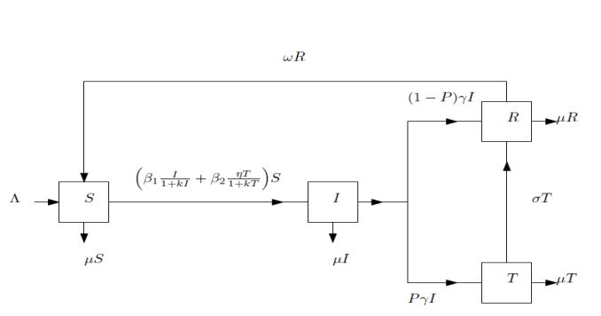
This model subdivides into four (4) compartments namely susceptible class (S), infective class (I), treated class (T) and recovered class (R). Thus, at time \(t\), the total population:
\begin{equation}\tag{A}
N(t)=S(t)+I(t)+T(t)+R(t)
\end{equation}
In Table 1 we give the detailed explanation of the parameters and variables used in model A
Figure 1. Schematic of diarrhoea model with saturated incidence.
Table 1. Description of Variables and Parameters of the model.
Parameters
Description
\(S\)
Susceptible
\(I\)
Infective
\(T\)
Treated class
\(R\)
Recovered class
\(\Lambda \)
Recruitment rate
\(\beta _{1} \)
Effective contact rate
\(\beta _{2} \)
Saturation treatment rate
\(\eta \)
Enhancement factor
\(P\)
Proportion of infected individuals joining either the class R or T
\(\gamma \)
Rate of treated individuals from infection
\(\sigma \)
Rate at which treated individuals move to recovered class
\(\omega \)
Rate at which recovered individuals move to susceptible class
\(\mu \)
The natural death rate in all compartments
\(\kappa \)
Educational adjustment
2.2. Model Equations
The following nonlinear system of dynamical equations was derived from model A:
In this section, we find the fundamental properties of the system (1), which is essential in the proof of the proceeding sections.
2.3.1. Positivity and Boundedness
The associated parameters of the system (1) with respect to the initial conditions are non-negative for all \(t>0\) and we prove this in the following procedures to get the results.
Lemma 1.
If \(\left\{S(0),I(0),T(0),R(0)\right\}\) and all associated parameters of the system are positive, then solutions \(S(t),I(t),T(t),R(t)\) are all positive \(\forall t>0\).
Proof.
Let
\[t_{1} =\sup \left\{t>0:S(t)\ge 0,I(t)\ge 0,T(t)\ge 0,R(t)\ge 0\right\}\]
From the first equation of (1), we have
\[\frac{dS}{dt} =\Lambda +\omega R-\mu S-\left(\beta _{1} \frac{I}{1+\kappa I} +\beta _{2} \frac{\eta T}{1+\kappa T} \right)S.\]
Since \(\left(\Lambda +\omega R\right)\ge 0\), then \(\frac{dS}{dt} \ge -\left(\mu +\phi \right)S,\)
where \(\phi =\left(\beta _{1} \frac{I}{1+\kappa I} +\beta _{2} \frac{\eta T}{1+\kappa T} \right)\).
Integrating both sides gives
\[\int _{0}^{t_{1} }\frac{dS}{dt} \ge -\int _{0}^{t_{1} }\left(\mu +\phi \right)dt ,\]
\[\left. \left(\ln \left|S(t)\right|\right)\right|_{0}^{t_{1} } \ge -\left(\mu +\phi \right)t_{1} ,\]
\[\left. S(t)\right|_{0}^{t_{1} } \ge e^{-\left(\mu +\phi \right)t_{1} } ,\]
\[S(t)\ge S(0)+e^{-\left(\mu +\phi \right)t_{1} } >0.\]
Next, we want to prove that \(I(t)>0\). From the second equation of (1), we have
Since \(\phi S\ge 0\), then we get
\[\frac{dI}{dt} \ge -\left(\mu +\gamma \right)I\]
Using the approach from (2), we get
\[\int _{0}^{t_{1} }\frac{dI}{I} \ge -\int _{0}^{t_{1} }\left(\mu +\gamma \right)dt ,\]
\[\left. \left(\ln \left|I(t)\right|\right)\right|_{0}^{t_{1} } \ge -\left(\mu +\gamma \right)t_{1} ,\]
\[\left. I(t)\right|_{0}^{t_{1} } \ge e^{-\left(\mu +\gamma \right)t_{1} } ,\]
\[I(t_{1} )\ge I(0)+e^{-\left(\mu +\gamma \right)t_{1} } >0.\]
Also we prove that \(T(t)>0\). From the third equation of (1), we have
\[\frac{dT}{dt} =P\gamma I-\left(\mu +\sigma \right)T\]
Since \(P\gamma I\ge 0\) then we have
\[\frac{dT}{dt} \ge -\left(\mu +\sigma \right)T. \]
This yields
\[\int _{0}^{t_{1} }\frac{dT}{T} \ge -\int _{0}^{t_{1} }\left(\mu +\sigma \right)dt \]
\[\left. \left(\ln \left|T(t)\right|\right)\right|_{0}^{t_{1} } \ge -\left(\mu +\sigma \right)t_{1} \]
\[\left. T(t)\right|_{0}^{t_{1} } \ge e^{-\left(\mu +\sigma \right)t_{1} } ,\]
\[T(t_{1} )\ge T(0)+e^{-\left(\mu +\sigma \right)t_{1} } >0.\]
Again, we prove that \(R(t)\ge 0\). From the fourth equation of Equation (1) we have
\[\frac{dR}{dt} =\left(1-P\right)\gamma I+\sigma T-\left(\mu +\omega \right)R.\]
Since \(\left(1-P\right)\gamma I+\sigma T\ge 0\). Then, we have
\[\frac{dR}{dt} \ge -\left(\mu +\omega \right)R. \]
Integrating gives us
\[\int _{0}^{t_{1} }\frac{dR}{R} \ge -\int _{0}^{t_{1} }\left(\mu +\omega \right)dt ,\]
\[\left. \left(\ln \left|R(t)\right|\right)\right|_{0}^{t_{1} } \ge -\left(\mu +\omega \right)t_{1} ,\]
\[\left. R(t)\right|_{0}^{t_{1} } \ge e^{-\left(\mu +\omega \right)t_{1} } ,\]
\[R(t)\ge R_{0} +e^{-\left(\mu +\omega \right)t_{1} } >0.\]
Also, the rate at which the total population varies over time is given by:
\begin{equation} \label{4}
\frac{dN}{dt} =\Lambda -\mu N
\end{equation}
(3)
Lemma 2.
The closed set \(\Omega =\left\{\left(S,I,T,R\right)\in {R}_{+}^{4} :0\le \left(S+I+T+R\right)\le \frac{\Lambda }{\mu } \right\}\) is positively invariant.
Proof.
Assume that \(\left\{S(t),I(t),T(t).R(t)\right\}\in {R}_{+}^{4} \forall t>0\). The equation (3) can be written as
\[\frac{dN}{\Lambda -\mu N} =dt\]
\[\int _{o}^{t}\frac{dN}{\Lambda -\mu N} =\int _{0}^{t}dt \]
\[N(t)=N(0)e^{-\mu t} +\frac{\Lambda }{\mu } \left(1-e^{-\mu t} \right)\]
\[{\mathop{\lim }\limits_{t\to \infty }} N(t)=\frac{\Lambda }{\mu } \]
if \(N(0)\le \frac{\Lambda }{\mu }\), then we have \(N(t)\le \frac{\Lambda }{\mu } ,\forall t>0\).
Moreover, if \(N(0)> \frac{\Lambda }{\mu }\), then the solution \(\left(S(t),I(t),T(t),R(t)\right)\) enter the closed set \(\Omega \) which affirms that \(\Omega \) is positively invariant. So, the region \(\Omega\) contains all solutions in \({R}_{+}^{4}\). Hence, it is sufficient to study the disease transmission dynamics under the dynamical system (1) in \(\Omega\).
3. Stability Analysis
In this section, we determine the disease free and endemic equilibrium points of Equation (1).
3.1. Disease Free Equilibrium (DFE)
The disease-free state denoted \(E^{0}\) is when there is no infection i.e \(I=T=R=0\) and is obtained by taking the right side of Equation (1) equal to zero. The corresponding disease-free equilibrium point is
\[E^{0} =\left(S^{0} ,0,0,0\right)=\left(\frac{\Lambda }{\mu } ,0,0,0\right).\]
3.2. Endemic Equilibrium (EE)
In this subsection, we determine the EE of Equation (1) denoted \(E^{1} =\left(S^{*} ,I^{*} ,T^{*} ,R^{*} \right)\). Taking the right side of Equation (1) equal to zero, the corresponding EE point is given by the following process.
The basic reproduction number denoted by \(R_{0}\) is defined as the average number of secondary infection generated by one infected individual into a completely susceptible population at a time t. It is a threshold parameter that allows us to predict whether the disease will die out or persist [11]. We calculate our \(R_{0}\) using the next generation matrix [15]. By referring to this approach, it is given by \(R_{0} =\rho \left(FV^{-1} \right)\) where \(\rho \left(A\right)\) denotes the spectral radius of a matrix \(A, F\) is new infection transfer terms, \(V\) is the non-singular matrix of the remaining transfer terms.
\[F=\left[\begin{array}{c} {\beta _{1} \frac{IS}{1+kI} +\beta _{2} \frac{\eta TS}{1+kT} } \\ {0} \end{array}\right].\]
Then the Jacobian of \(F\) at \(E^{0} \) is
\[F=\left[\begin{array}{cc} {\frac{\Lambda \beta _{1} }{\mu } } & {\frac{\eta \Lambda \beta _{2} }{\mu } } \\ {0} & {0} \end{array}\right].\]
Let \(V\) denotes the Jacobian of \(v\) at \(E^{0} \),
\[v=\left[\begin{array}{c} {\left(\mu +\gamma \right)I} \\ {-P\gamma I+\left(\mu +\sigma \right)T} \end{array}\right].\]
\[V=\left[\begin{array}{cc} {\left(\mu +\gamma \right)} & {0} \\ {-P\gamma } & {\left(\mu +\sigma \right)} \end{array}\right].\]
So, below is the next generation matrix obtained, and it allows us to find the basic reproduction number
\[A=FV^{-1} =\left[\begin{array}{cc} {\frac{\Lambda \beta _{1} }{\mu \left(\mu +\gamma \right)} +\frac{p\gamma \eta \Lambda \beta _{2} }{\mu \left(\mu +\gamma \right)\left(\mu +\sigma \right)} } & {\frac{\eta \Lambda \beta _{2} }{\mu \left(\mu +\sigma \right)} } \\ {0} & {0} \end{array}\right].\]
\(R_{0} \) is the leading eigenvalue of the next generation matrix,
\[R_{0} =\frac{\Lambda \left(\mu \beta _{1} +\sigma \beta _{1} +P\gamma \eta \beta _{2} \right)}{\mu \left(\mu +\gamma \right)\left(\mu +\sigma \right)} .\]
3.4. Local Stability of Disease-Free Equilibrium (\(E^{0} \))
In this subsection, we prove the local stability of the disease-free equilibrium of Equation (1) .
Evaluating the Jacobian at \(E_{0}\). Hence, we obtain
\[J_{E^{0} } =\left[\begin{array}{cccc} {-\mu } & {-\beta _{1} \frac{\Lambda }{\mu } } & {-\beta _{2} \frac{\eta \Lambda }{\mu } } & {\omega } \\ {\phi } & {\beta _{1} \frac{\Lambda }{\mu } -\left(\mu +\gamma \right)} & {\beta _{2} \frac{\eta \Lambda }{\mu } } & {0} \\ {0} & {P\gamma } & {-\left(\mu +\sigma \right)} & {0} \\ {0} & {\left(1-P\right)\gamma } & {\sigma } & {-\left(\mu +\omega \right)} \end{array}\right].\]
Here, we evaluate the Jacobian at \(E^{0}\) and identity matrix to get the eigenvalues, that is,
\[\left|J_{E^{0} } -\lambda I\right|=\left|\begin{array}{cccc} {-\mu -\lambda } & {-\beta _{1} \frac{\Lambda }{\mu } } & {-\beta _{2} \frac{\eta \Lambda }{\mu } } & {\omega } \\ {\phi } & {\beta _{1} \frac{\Lambda }{\mu } -\left(\mu +\gamma \right)-\lambda } & {\beta _{2} \frac{\eta \Lambda }{\mu } } & {0} \\ {0} & {P\gamma } & {-\left(\mu +\sigma \right)-\lambda } & {0} \\ {0} & {\left(1-P\right)\gamma } & {\sigma } & {-\left(\mu +\omega \right)-\lambda } \end{array}\right|=0.\]
Then \(\lambda _{1} =-\mu < 0\) and \(\lambda _{2} =-\left(\mu +\omega \right)< 0\).The remaining eigenvalues can be obtained by solving
\[H=\left|\begin{array}{cc} {\beta _{1} \frac{\Lambda }{\mu } -\left(\mu +\gamma \right)-\lambda } & {\beta _{2} \frac{\eta \Lambda }{\mu } } \\ {P\gamma } & {-\left(\mu +\sigma \right)-\lambda } \end{array}\right|=0.\]
Then we get the following characteristic equation
\[\lambda ^{2} +\left(2\mu +\gamma +\sigma -\beta _{1} \frac{\Lambda }{\mu } \right)\lambda +\mu ^{2} +\left(\sigma +\gamma -\beta _{1} \frac{\Lambda }{\mu } \right)\mu +\left(\gamma -\beta _{1} \frac{\Lambda }{\mu } \right)-\beta _{2} \frac{P\gamma \eta \Lambda }{\mu } =0.\]
We have a form of quadratic equation, that is,
\[P\left(\lambda \right)=\lambda ^{2} +a_{1} \lambda +a_{2} =o,\]
where
\(a_{1} =\left(\mu +\gamma \right)+\left(\mu +\sigma \right)-\beta _{1} \frac{\Lambda }{\mu }\) and \(a_{2} =\left(\mu +\sigma \right)\left(\mu +\gamma \right)\left[1-R_{0} \right]\).
If \(R_{0} 0\) and if \(R_{0} < 1\), then \(\beta _{1} \frac{\Lambda }{\mu \left(\mu +\gamma \right)} 0\). Hence the disease-free equilibrium is locally asymptotically stable if \(R_{0} < 1\).
3.5. Global Stability of the Disease Free Equilibrium (\(E^{0}\))
Theorem 4. The disease free equilibrium is globally stable in \(\Omega\) if \(R_{0} < 1\), where \(\Omega\) is a feasible region of Equation (1) and contains all solutions in \({R}_{+}^{4}\) as shown in the previous proof.
Again, we prove that the disease-free equilibrium is globally asymptotically stable, using the approach of Castillo – Chavez [13].
Proof.
We group Equation (1) into two compartments, that is, uninfected and infected individuals, given by
\[\left. \begin{array}{l} {a_{1} :\frac{dX}{dt} =F(X,Z)} \\ {a_{2} :\frac{dZ}{dt} =G(X,Z),G(X,0)=0} \end{array}\right\}. \]
Where \(X=(S,R),Z=(I,T)\) with \(X\in {R}_{+}^{2}\) representing the uninfected individuals and \(Z\in {R}_{+}^{2}\) representing infected individuals including the latent and infectious.
Let us denote the disease-free equilibrium point by
We can see that \(\lambda _{1} =-U,\lambda _{2} =-\left(\mu +A\right),\left(a_{1} ,a_{2} \right)>0\). Then, all roots of the characteristic equation above have negative real part. Therefore, the endemic equilibrium of Equation (1) is locally asymptotically stable if \(R_{0} >1\).
4. Numerical simulations
In this section, we would show numerical simulations for the proposed Model A. This analysis was carried out in Python with the following initial conditions and parameter values \(S = 600; I = 100; T = 0; R = 0.\)
In Table 2 we give the detailed explanation of the parameters, variable and values used in the Model.
Using Python software, we were able to get the following results. The plots are considered for a deterministic model ‘SITR’, we computed basic reproduction number \(R_{0}\) as an important threshold parameter that has played great role to predict if the diarrhea disease will die out or persist within the population. The detailed explanations of parameters used are under each figure.
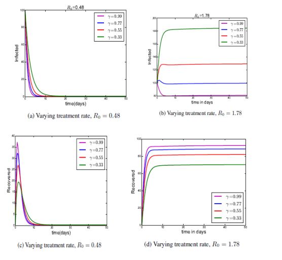
Figure 2..
Figure 2 shows the numerical simulation solutions of the system model A with different \(R_{0}\) values with the following parameter values \(\Lambda = 45; \beta _{1} = 0:0035; \beta _{2} = 0:05; \eta = 0:02; P = 0:04; \gamma = 0:7; \sigma = 0:9; \omega = 0:8; \mu = 0:063; k = 0:012.\)
From figure 2a the infected individuals decrease to zero. This means that, the more saturation treatment the more disease dies out of the population. From Figure 2b as long as we reduce the education and saturation treatment rate, the infected class increases, however when we increase the rate at which individuals are treated to 99%, the infected class goes to zero i.e the disease dies out as time t increases. This shows us that the saturation treatment has an effect to the spread of diarrhea.
From figure 2c , we have seen that as long as we increase the education k, then saturation treatment rate; has an effect on treatment as \(\beta _{2} \mathrm{>}\mathrm{>}\beta _{1}\) increasingly. Thus, by varying the treatment, the recovered individuals increase from 19-37 in 1 day. This means that, the more saturation treatment the more people recover, and consequently the disease will die out of the population. From Figure 2d with \(R_{0} \mathrm{>} 1\) means that the diarrhea disease will increase and cannot be eradicated from the population and it is expected that the disease will remain endemic.
5. Conclusion
In this paper, we have analysed the disease-free equilibrium (\(E_{0}\)), the endemic equilibrium
(\(E_{1}\)), and the basic reproduction number (\(R_{0}\)). We have shown the local and global stability of the disease-free equilibrium point. We have shown that the endemic equilibrium point is locally
asymptotically stable if \(R_{0}>1\) and this means that the diarrhoea disease will persist in population. We have also seen that if \(R_{0}< 1\) the diarrhoea disease will die out of the population after some time.
Furthermore, we used python to carry out numerical simulations, and the results show that the maximum possible treatment (saturation treatment rate) affect the dynamics of diarrhea disease. The more saturation treatment, given to individuals, the more the disease dies out of the population. Treatment mention in this project means, giving the infected population the anti-diarrhoea drugs that is: Imodium (loperamide) and Pepto-Bismol or Kaopectate (bismuth subsalicylate). These drugs are helpful in stopping an occasional bout of diarrhoea especially traveler's diarrhoea, which may result from ingesting contaminated food or water while abroad.
We recommend the health policy makers that the drugs should be made available to consumers at saturation treatment rate of 99% at a very low cost on time to reduce the dynamical spread of diarrhoea in a community and to avoid epidemics.
Author Contributions
All authors contributed equally to the writing of this paper. All authors read and approved the
final manuscript.
Competing Interests
The author(s) do not have any competing interests in the manuscript.
References
Ardkaew, J., & Tongkumchum, P. (2009). Statistical modelling of childhood diarrhea in northeastern Thailand. Southeast Asian Journal of Tropical Medicine and Public Health, 40(4), 807-815. [Google Scholor]
Bennett, J. E., Dolin, R., & Blaser, M. J. (2014). Principles and practice of infectious diseases (Vol. 1). Elsevier Health Sciences. [Google Scholor]
Black, R. E. (1993). Epidemiology of diarrhoeal disease: implications for control by vaccines. Vaccine, 11(2), 100-106.[Google Scholor]
Auld, H., MacIver, D., & Klaassen, J. (2004). Heavy rainfall and waterborne disease outbreaks: the Walkerton example. Journal of Toxicology and Environmental Health, Part A, 67(20-22), 1879-1887. [Google Scholor]
Cherry, B. R., Reeves, M. J., & Smith, G. (1998). Evaluation of bovine viral diarrhea virus control using a mathematical model of infection dynamics. Preventive Veterinary Medicine, 33(1-4), 91-108.[Google Scholor]
Diekmann, O., Heesterbeek, J. A. P., & Metz, J. A. (1990). On the definition and the computation of the basic reproduction ratio \(R_{0}\) in models for infectious diseases in heterogeneous populations. Journal of mathematical biology, 28(4), 365-382. [Google Scholor]
Fuller, A. T. (1968). Conditions for a matrix to have only characteristic roots with negative real parts. Journal of Mathematical Analysis and Applications, 23(1), 71-98. [Google Scholor]
Gatto, M., Mari, L., & Rinaldo, A. (2013). Leading eigenvalues and the spread of cholera. SIAM News, 46(7). [Google Scholor]
Githeko, A. K., Lindsay, S. W., Confalonieri, U. E., & Patz, J. A. (2000). Climate change and vector-borne diseases: a regional analysis. Bulletin of the World Health Organization, 78, 1136-1147. [Google Scholor]
Chaturvedi, O., Jeffrey, M., Lungu, E., & Masupe, S. (2017). Epidemic model formulation and analysis for diarrheal infections caused by salmonella. Simulation, 93(7), 543-552. [Google Scholor]
Jose, M. V., & Bobadilla, J. R. (1994). Epidemiological model of diarrhoeal diseases and its application in prevention and control. Vaccine, 12(2), 109-116.[Google Scholor]
Ardkaew, J., & Tongkumchum, P. (2009). Statistical modelling of childhood diarrhea in northeastern Thailand. Southeast Asian Journal of Tropical Medicine and Public Health, 40(4), 807-815.
[Google Scholor]
Hunter, P. R. (2003). Climate change and waterborne and vector-borne disease. Journal of applied microbiology, 94, 37-46.[Google Scholor]
Mushayabasa, S. (2012). A simple epidemiological model for typhoid with saturated incidence rate and treatment effect. International Journal of Biological, Veterinary, Agricultural and Food Engineering, 6(6), 688-695. [Google Scholor]
Hirsch, M. W., Smale, S., & Devaney, R. L. (2012). Differential equations, dynamical systems, and an introduction to chaos. Academic press. [Google Scholor]