Numerical solution of boundary layer flow of MHD nanofluid over a stretching surface with chemical reaction and viscous dissipation effects

1. Introduction

The study of flow and heat transfer generated by means of stretching medium has plenty of significance in numerous industrialized developments, (e.g., in the process of rubber and plastic sheets manufacturing, upgrading the solid materials like crystal, turning fibers etc.). The most widely used coolant liquid among them is water. In above cases, flow and heat transfer investigation is of major importance because final product quality be determined to bulk level on the basis of coefficient of skin friction and heat transfer surface rate. Numerous investigators talked over different traits of stretching flow problem. Some of them are Crane [1], Chaim [2], Liao and Pop [3], Khan and Sanjayanand [4], and Fang et al. [5].

Currently, in the fields of engineering and fluid science, heat transfer and boundary layer flow of nanofluid are the thrust areas of research. Many researchers examined the convective boundary layer flow of nanofluid past a stretched sheet. In future, advancement in nano-technology is expected for making unbelievable changes in our lives. A very big number of researchers are working in this area due to its great use in the engineering and its linked areas. In the process of air cleaning, development of microelectronics, safety of nuclear reactors etc., heat and mass transfer of thermophoretic magnetohydrodynamic flow consumes prospective uses. Choi [6] was the first who introduced the idea of ``nanofluids" and presented the report on the heat transfer properties of nano-fluids. The thorough exposure on thermophoretic flow was examined by Derjaguin and Yalamov [7]. Heat and mass transfer of MHD thermophoretic stream above plane surface was also studied by Issac and Chamka [8]. Thermophoresis effect on aerosol particles was investigated by Tsai [9].

In fluid temperature, no doubt, viscous dissipation produces a considerable ascend. This would happen because of change in kinetic motion of fluid into thermal energy. Viscous dissipation is unavoidable in case of flow field in high gravitational field. Viscous flow past a nonlinearly stretching sheet was deliberated by Vajravelu [10]. For external natural convention flow over a stretching medium, the effect of viscous dissipation was also studied by Mollendroff and Gebhart [11], whereas the impact of Joule heating and viscous dissipation on the forced convection flow with thermal radiation was presented by Duwairi [12].

The chemical reaction with the diffusion of species for the boundary layer fluid have numerous applications in atmosphere pollution, water, fluids relevant to atmosphere and many other problems of chemical engineering. For boundary layer laminar flow of reactive chemically species with the diffusion which are used by a body over the surface considered by Chamber and Young [13]. For non-Newtonian fluids and their solution for the species of diffusion with chemical reactive in a flow over a stretching sheet with porous medium reported by Akyildiz et al. [14]. Cortell [15] also discuss the two types of viscoelastic fluid over a porous stretching sheet with the chemically reactive species. Hiemenz flow through porous media considered by Chamka and Khaled [16] with the presence of magnetic field. Heat transfer with steady condition considered by Sriramalu et al. [17] for incompressible viscous fluid with porous type species over a stretching surface. Khan et al. [18] discussed MHD viscoelastic fluid, transfer of mass and heat over a permeable stretching surface with stress work and energy dissipation. The fluid on stretching surface close with stagnation-point discussed by Tripathy et al. [19]. Seddeek and Salem [20] observed that the mass and heat transfer distribution on stretching type surface with thermal diffusivity and variable viscosity.

In this article, we provide a review study of M. G. Reddy [21] and then extend the flow analysis with chemical reaction parameter and viscous dissipation properties. There are many practical applications for the boundary layer flow over a stretching sheet in the presence of chemical reaction parameter and viscous dissipation effects.

2. Problem formulation

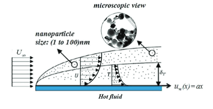
Let us consider the numerical investigation of MHD boundary layer flow of an incompressible nanofluid. The flow is two-dimensional, steady, laminar, viscous flow of an electrically conducting electrically conducting fluid towards a stretching surface with chemically reactive species undergoing chemical reaction is considered. The schematic diagram of the system under investigation is shown in the Figure 1.

The plate has been stretched with velocity \(u_w\left(x\right)=ax\), \(\left(a>0\right)\) along \(x-\) direction. In addition, fluid is flowing in the presence of magnetic field. The magnetic field is supposed to be applied along the \(y\mathrm{-}\)direction. The temperature at surface is \(T_f\), \(u_w,\) \(C_w\) represent fluid velocity, nanoparticle concentration at surface respectively.

The following system of equations are incorporated for mathematical model [21]. shows that in the presence of magnetic field over the surface, the governing equations of conservation of momentum, energy, mass and nanoparticle fraction, under the boundary layer approximation, are as follows:

• Continuity equation:
  \begin{equation}\label{e1} \frac{\partial u}{\partial x}+\frac{\partial v}{\partial y}=0 \end{equation}

  (1)
• Momentum equation:
  \begin{equation}\label{e2} u\frac{\partial u}{\partial x}+v\frac{\partial u}{\partial y}=-\frac{1}{{\rho }_f}\frac{\partial p}{\partial x}-\frac{\sigma B^2_0\left(x\right)}{{\rho }_f}\left(u\right)+\nu \left(\frac{{\partial }^2u}{\partial x^2}+\frac{{\partial }^2u}{\partial y^2}\right), \end{equation}

  (2)
  \begin{equation}\label{e3} u\frac{\partial v}{\partial x}+v\frac{\partial v}{\partial y}=-\frac{1}{{\rho }_f}\frac{\partial p}{\partial y}-\frac{\sigma B^2_0\left(x\right)}{{\rho }_f}\left(v\right)+\nu \left(\frac{{\partial }^2u}{\partial x^2}+\frac{{\partial }^2u}{\partial y^2}\right), \end{equation}

  (3)
• Energy equation:
  \begin{equation}\label{e4} u\frac{\partial T}{\partial x}+v\frac{\partial T}{\partial y}=\frac{\mu }{C_p}{\left(\frac{\partial u}{\partial y}\right)}^2+\alpha \frac{\partial ^2T}{\partial y^2}+\mathrm{\tau }\left[D_B\frac{\partial C}{\partial y}\frac{\partial T}{\partial y}+\frac{D_T}{T_{\infty }}{\left(\frac{\partial T}{\partial y}\right)}^2\right]-\frac{\alpha }{{\rho }_f}\left(\frac{\partial q_r}{\partial y}\right) \end{equation}

  (4)
• Concentration equation:
  \begin{equation}\label{e5} u\frac{\partial C}{\partial x}+v\frac{\partial C}{\partial y}=D_B\frac{{\partial }^2C}{\partial y^2}+\frac{D_T}{T_{\infty }}\frac{{\partial }^2C}{\partial y^2}-k_0(C-C_{\infty }) \end{equation}

  (5)

where \(u\) and \(v\) are the components of velocity respectively in the \(x\) and \(y\) directions, \(p\) is the fluid pressure, \({\rho }_f\) is the density of base fluid, \({\rho }_p\) is the density of the particles, \(\nu \) is the kinematic viscosity of the base fluid, \(\sigma\) is electrical conductivity, \(\rho \) is density, \(T\) is temperature, \(\alpha \) is thermal diffusivity, \(\tau =\frac{{\left(\rho c\right)}_p}{{\left(\rho c\right)}_f}\) is the ratio of nanoparticle heat capacity and the base fluid heat capacity, \(D_B\) is Brownian diffusion coefficient, \(D_T\) is thermophoretic diffusion coefficient, \(\mu \) is dynamic viscosity, \(c\) is specific heat at constant pressure.

The boundary conditions for Equations (1), (2), (3), (4) and (5) are The radiative heat flux \(q_r,\) by using the Rosseland approximation for radiation, can be written as where \({\sigma }^*\) and \(k^*\) stand for the Stefan-Boltzmann constant and coefficient of mean absorption. Expansion of \(T^4\) about \(T_{\infty }\) by making use of Taylor's series is: Disregarding the higher order terms, we have \[T^4=T^4_{\infty }+4T^3_{\infty }\left(T-T_{\infty }\right)\] Using (8) in (6) and the differentiate with respect to \(y\), we get We use similarity transformation to solve Equations (1), (2), (3), (4) and (5) the velocity component of stream function which is defined as So, we have where prime shows differentiation with respect to \(\eta \). Using Equation (11) in Equation (1) that will be satisfied, also using Equations (6)-(12) in Equations (2)-(4), we will get the following ordinary differential equations. with the boundary conditions The dimensionless constants \(M\), \(S\),\(\ R,\) \(\mathrm{A}\), \(\mathrm{Pr}\), \(Nb\), \(Nt\), \(Ec\),\(\ Le\), \(\gamma \), \(Bi\) represent the magnetic parameter, a suction parameter, the radiation parameter, the velocity slip parameter, the Prandtl number, the Browian motion parameter, the thermophoresis parameter, the Eckert number, the Lewis number, the chemical rate parameter, the Biot number respectively, which are defined as \[\ M=\frac{\sigma B^2_0}{\rho a},S=-\frac{v_w}{\sqrt{a\nu }},\ A=L\left(\sqrt{\frac{a}{\nu }}\right),\ \ R=\frac{-4{T^3_{\infty }\sigma }^*}{3k^*k},\ Pr=\frac{\nu }{\alpha },Nb=\frac{\tau D_B\left(C_w-C_{\infty }\right)}{\nu },\] \[\ Nt=\frac{\tau D_T\left(T_f\mathrm{-}T_{\mathrm{\infty }}\right)}{\nu T_{\mathrm{\infty }}},Ec=\frac{u^2_w}{{\rho }_f\left(T_f\mathrm{-}T_{\mathrm{\infty }}\right)},\ Le=\frac{\nu }{D_B},\ \gamma =\frac{k_0U\left(C_w-C_{\infty }\right)}{\nu },\ Bi=\frac{h{\left({\nu }/{a}\right)}^{{1}/{2}}}{k}. \] The quantities of practical interest in this study are the Nusselt number \({Nu}_x\), the skin friction coefficient\(\mathrm{\ }C_f\), and the Sherwood number \({Sh}_x\), respectively. These are expressed as: where, \({\tau }_w\) is the shear stress,\(\ q_m\) is the wall mass flux from the surface, and \(q_w\) is the heat flux at the wall surface, given by: Using the dimensionless variables, we get where \({Re}_x\) denotes the Reynolds number and is expressed as: \[{Re}_x=\frac{xU_w(x)}{v} .\]

3. Method for solution

The set of non-linear coupled differential equations (14), (15) and (16) with the conditions (17) is solved numerically in the following manner. Firstly, it is noticed that heurist infinity for the independent variable chosen as \({\eta }_{max}\). The comment on the choice on the \({\eta }_{max}\), for solving is presented at the end of the section. Equation (13) is solved with \(f^{''}\left(0\right)=r\), assumed number using the initial conditions \(r\) is iteratively found using Newton's method using \(F'\left({\eta }_{max}\right)=\frac{\partial f'(max)}{\partial \alpha }\) which is obtain by solving, with After finding \(f(\eta )\) we solved the equations \(15\) \& \(16\) with the initial conditions. Associated boundary conditions in Equation (17) can be written as Here \(\ p_1=\theta \left(0\right)and\ p_2\left(0\right)={\beta }'(0)\). \(p_1,p_2\) are to be found satisfying end conditions \(y_1\to 0,y_3\to 0\) as \(\eta \to \infty \). Adams Moultan fourth order method (with the corresponding predictor) is used to solve the initial value problem. Assumed values of \(p_1\ \)and \(p_2\) are corrected using Newton method. Derivatives of \(\theta (\infty ,p_1,p_2)\) and \(\ \phi (\infty ,p_1,p_2)\) with respect to any parameter \(p(p_1or\ p_2\ )\) are found by solving the equation which are obtained by differentiating system (21). \(Y_i=\frac{\partial y_i}{\partial p}\ \)for all \(i=1,2,3,4\). These equations are \[Y'_1=Y(2),\] \[Y'_2=\frac{-Pr}{\left(1+\frac{4Ra}{3}\right)}[FF(I)Y\left(2\right)+Nb\left(y\left(2\right)Y\left(4\right)-Y\left(2\right)y\left(4\right))+2Nty\left(2\right)Y\left(2\right)\right],\] \[Y'_3=Y(4),\] \[Y'_4==-LeFF\left(I\right)y\left(4\right)-\frac{Nt}{Nb}Y'_2+Le\gamma y(3)\] This system is solved with three different sets of initial conditions \(y_i\left(0\right)=0\) for all \(i=1,2,3,4\). Newton's method is It may be noticed that the choice of initial guess of \(p_1,p_2\) is very crucial. Once we obtain solution for a set of physical parameters, a single parameter changed slightly to achieve convergence of newton's method. The choice of \({\eta }_{max}=6\ \)was more than enough for end condition. The convergence criteria is chosen to be successive value agree up to 3 significant digits.

4. Results with discussion

The objective of this section, the numerical results have been displayed in the form of graphs and tables. The computations are carried out for various values of the magnetic parameter \(M\), Prandtl number \(Pr\), a radiation parameter \(R\), a Brownian motion parameter \(Nb\) , a thermophoresis parameter \(Nt\) , a Lewis number \(Le\), Eckert number \(Ec\), slip parameter \(A\) , chemical reaction parameter \(\gamma \) and the impact of these parameters on velocity \(f'\), temperature \(\theta \) and concentration \(\beta \) have been analyzed.

For the validity of our results, the skin friction factor, the local Nusselt number and Sherwood number have been compared with those already published in literature as shown in Tables 1 and 2. From tables it can be seen that the results achieved by the present code are found convincingly very closed to the published results [21].

Table 1. Comparison of results of skin friction coefficient \(-f^"(0)\) for various values of \(M,\ S\)\textit{ }and \(A\)

\(M\)	\(S\)	\(A\)		\(-f^"(0)\)
			M. G. Reddy [21]	Present value
0.5	0.2	0.1	1.13992	1.136756
1.0	0.2	0.1	1.28430	1.282955
0.5	0.5	0.1	1.26830	1.265184
0.5	0.2	0.5	0.800331	0.8066351

Table 2. Comparison of results of local Nusselt number \(-{\theta }'(0)\) and Sherwood number \(-{\beta }'(0)\)

\(Nt\)	\(Nb\)		\(-{\theta }'(0)\)	\(-{\beta }'(0)\)
		M. G. Reddy [21]	Present value	M. G. Reddy [21]	Present value
0.1	0.1	0.0840676	0.0822515300	2.96584	2.9588820000
0.5	0.1	0.0813944	0.0792839800	3.00253	3.0008590000
0.1	0.5	0.0838497	0.0819882600	2.79651	2.7606710000
0.5	0.5	0.0811044	0.0789362500	2.97637	2.9675340000

In every one of these estimations, we have considered \(Pr=2,\ M=2,\ R=2,\ Nb=Nt=S=A=Ec=\gamma =0.5,\ Bi=0.1\) and \(Le=5.\)

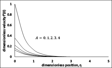
4.1. Impact of slip parameter (A)

The effect of slip parameter \(A\) on the dimensionless velocity profile \(f'(\eta )\) is presented in Figure 2. Increasing the values of the slip parameter \(A\) reduces the velocity field and particular boundary thickness as depicted in Figure 2.

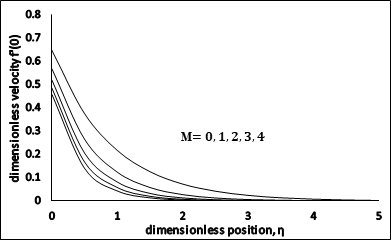
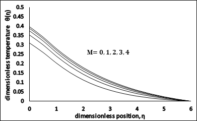
4.2. Impact of Magnetic parameter \(\left(M\right).\)

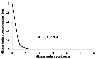
Figure 3, Figure 4 and Figure 5 shows the variations in the velocity profile \(f'(\eta )\), energy profile \(\theta (\eta )\) and dimensionless concentration profile \(\beta (\eta )\) for different estimations of Magnetic Parameter \(M\). It is analyzed that the temperature profile \(\theta (\eta )\), concentration profile \(\beta (\eta )\) and thermal boundary layer thickens are increasing functions of Magnetic Parameter, however on the opposite side velocity profile \(f'(\eta )\) decreases when we increase Magnetic Parameter \(M\). The reason beyond this electrically conducting fluid produces a resistive force known as Lorentz force, which opposes the flow and has a tendency to make the fluid motion slow down in the boundary layer and therefore reduces the profile of velocity whereas its temperature \(\theta (\eta )\) increases with the increase in magnetic parameter.

4.3. Impact of suction parameter \(\left(S\right)\).

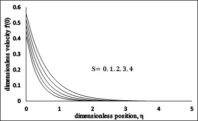
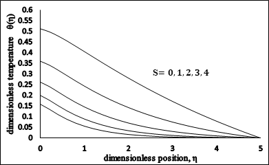
The impact of the section parameter \(S\) on the dimensionless velocity profile \(f'(\eta )\) is presented in Figure 6. Velocity profile diminishes and accompanied with boundary layer width increases for gradually growing values of the suction parameter \(S\). Figure 7 displays the variation of temperature with suction parameter. As the values of suction parameter\(\ S\) increase, the temperature graph is decreasing. Moreover, the thermal boundary layer thickness and surface temperature is also decreasing. Figure 8 shows that by increasing suction parameter \(S\), concentration profile decreases. By an increasing in the suction, concentration profile as well as boundary layer thickness decrease.

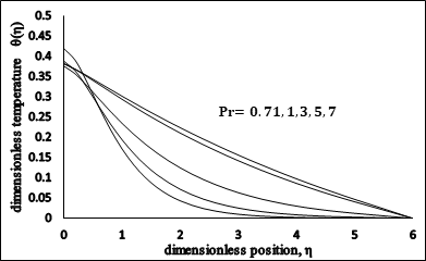
4.4. Impact of Prandtl number \(\left(Pr\right)\).

Figure 9 presents that an elevation in Prandtl number \(Pr\) shows a reduction in the temperature profile \(\theta (\eta )\). Obviously, greater Prandtl number \(Pr\ \)has weaker thermal diffusivity due to which low range temperature is seen in Figure 8. This indicates resection in energy exchange ability and finally it causes an reduction in thermal boundary surface.

4.5. Impact of Radiation parameter \(\boldsymbol{\ }\left(R\right)\).

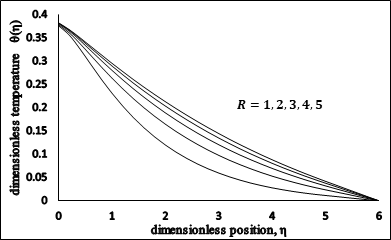
The influence of radiation parameter on profile of temperature distribution is displayed in Figure 10. From the figure it is observed that by increasing the radiation parameter, temperature profile decreases significantly. It is because of the fact that the increasing values of radiation parameter lead to decrease the thickness of the boundary layer and enhance the heat transfer rate with chemical effect on the melting surface.

4.6. Impact of Convective Heating \(\left(Bi\right)\).

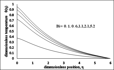
Figure 11 describes the effect of the convective heating which is also known as the Biot number on the temperature profile \(\theta (\eta )\). Numerically, it can be calculated by dividing the convection on the surface to the conduction into the surface of an object. When \(Bi\) increases, it causes increase in the temperature on surface which sequels in the thickening of the thermal boundary layer.

4.7. Impact of Brownian motion and the thermophoresis on unitless energy profile

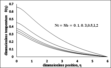
Figure 12 show the impact of Brownian motion and the thermophoresis parameters on the temperature distributions\(\ \theta (\eta )\) in the thermal boundary layer. Thermophoresis is a component that drives small materials away from hot layer to the cooler end. It is noticed that as thermophoresis parameter increases the thermal boundary layer thickness increases and the temperature gradient at the surface decrease (in absolute value) as both \(Nb\) and \(Nt\) increase.

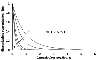
4.8. Impact of Lewis number \(\left(\boldsymbol{Le}\right)\)

Lewis number \(Le\) is decreasing function of \(\beta (\eta )\). Increase Lewis number may decrease Brownian diffusion coefficient because Lewis number is the ratio of momentum diffusivity to Brownian diffusion coefficient, shown in Figure 13.

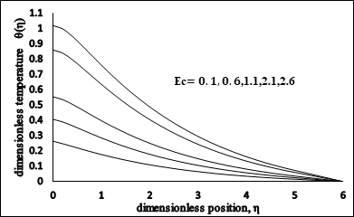
4.9. Impact of Eckert number \(\left(Ec\right)\).

Figure 14 displays the influence of Eckert number \(Ec\) on the energy profile. Energy profile increases when the Eckert number is increased. Due to friction, the heat energy is kept in owing to accelerating values of Eckert number, which results in the enhancement of the temperature profile.

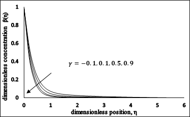
4.10. Impact of chemical reaction parameter

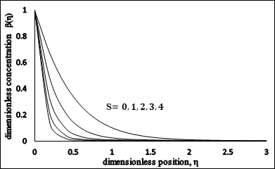
Figure 15 explains the influence of the chemical reaction parameter on the profile of concentration. It is noted that increasing values of chemical reaction parameter concentration as well as the thickness of concentration decrease. It is because of the fact that the chemical reaction in this system results in chemical dissipation and therefore results in decrease in the profile of concentration. The most significant influence is that chemical reaction tends to increase the overshoot in the concentration profiles and their associated boundary layer.

5. Conclusion

From the above discussion, we can make the following conclusions.

1. Higher values of \(M\) yield an increment in the energy profile and Concentration profile whereas an opposite effect has noticed for the velocity profile.
2. By increasing in the suction parameter \(S\), velocity profile increases whereas temperature profile decreases with an increase in suction while due to increasing blowing, it increases.
3. The thickness of concentration boundary layers reduces due to increasing in the suction parameter.
4. Increase of Prandtl number \(Pr\) and Radiation parameter \(R\) causes decrease in temperature profile.
5. Temperature increase by enlarging thermophoresis parameter \(Nt\) and Brownian motion parameter \(Nb\)
6. For larger values of Lewis number \(Le\) and chemical reaction parameter \(\gamma \) , concentration field \(\beta \left(\eta \right)\) shows decreasing behavior.
7. Temperature profile will increase due to increases in the Eckert number.

Acknowledgments

The authors wishes to express his profound gratitude to the reviewers for their useful comments on the manuscript.

Author Contributions

All authors contributed equally to the writing of this paper. All authors read and approved the final manuscript.

Competing Interests

The author(s) do not have any competing interests in the manuscript.

References

Crane, L. J. (1970). Flow past a stretching plate. Zeitschrift für angewandte Mathematik und Physik ZAMP, 21(4), 645-647.[Google Scholor]
Chiam, T. C. (1995). Hydromagnetic flow over a surface stretching with a power-law velocity. International Journal of Engineering Science, 33(3), 429-435. [Google Scholor]
Liao, S. J., & Pop, I. (2004). Explicit analytic solution for similarity boundary layer equations. International Journal of Heat and Mass Transfer, 47(1), 75-85. [Google Scholor]
Khan, S. K., & Sanjayanand, E. (2005). Viscoelastic boundary layer flow and heat transfer over an exponential stretching sheet. International Journal of Heat and Mass Transfer, 48(8), 1534-1542.[Google Scholor]
Fang, T., Chia-fon, F. L., & Zhang, J. (2011). The boundary layers of an unsteady incompressible stagnation-point flow with mass transfer. International Journal of Non-Linear Mechanics, 46(7), 942-948. [Google Scholor]
Choi, S. U., & Eastman, J. A. (1995). Enhancing thermal conductivity of fluids with nanoparticles (No. ANL/MSD/CP-84938; CONF-951135-29). Argonne National Lab., IL (United States). [Google Scholor]
Derjaguin, B. V., & Yalamov, Y. (1965). Theory of thermophoresis of large aerosol particles. Journal of colloid science, 20(6), 555-570.[Google Scholor]
Chamkha, A. J., & Issa, C. (2000). Effects of heat generation/absorption and thermophoresis on hydromagnetic flow with heat and mass transfer over a flat surface. International Journal of Numerical Methods for Heat & Fluid Flow, 10(4), 432-449.[Google Scholor]
Tsai, R. (1999). A simple approach for evaluating the effect of wall suction and thermophoresis on aerosol particle deposition from a laminar flow over a flat plate. International communications in heat and mass transfer, 26(2), 249-257.[Google Scholor]
Vajravelu, K. (2001). Viscous flow over a nonlinearly stretching sheet. Applied mathematics and computation, 124(3), 281-288.[Google Scholor]
Gebhart, B., & Mollendorf, J. (1969). Viscous dissipation in external natural convection flows. Journal of fluid Mechanics, 38(1), 97-107.[Google Scholor]
Duwairi, H. M. (2005). Viscous and Joule heating effects on forced convection flow from radiate isothermal porous surfaces. International Journal of Numerical Methods for Heat & Fluid Flow, 15(5), 429-440.[Google Scholor]
Chambré, P. L., & Young, J. D. (1958). On the diffusion of a chemically reactive species in a laminar boundary layer flow. The Physics of fluids, 1(1), 48-54.[Google Scholor]
Akyildiz, F. T., Bellout, H., & Vajravelu, K. (2006). Diffusion of chemically reactive species in a porous medium over a stretching sheet. Journal of Mathematical Analysis and Applications, 320(1), 322-339.[Google Scholor]
Cortell, R. (2005). Flow and heat transfer of a fluid through a porous medium over a stretching surface with internal heat generation/absorption and suction/blowing. Fluid Dynamics Research, 37(4), 231.[Google Scholor]
Chamkha, A. J., & Khaled, A. R. A. (2000). Similarity solutions for hydromagnetic mixed convection heat and mass transfer for Hiemenz flow through porous media. International Journal of Numerical Methods for Heat & Fluid Flow, 10(1), 94-115.[Google Scholor]
Sriramalu, A., Kishan, N., & Anand, R. J. (2001). Steady flow and heat transfer of a viscous incompressible fluid flow through porous medium over a stretching sheet. Journal of Energy Heat Mass Transfer, 23, 483-495.[Google Scholor]
Khan, S. K., Abel, M. S., & Sonth, R. M. (2003). Visco-elastic MHD flow, heat and mass transfer over a porous stretching sheet with dissipation of energy and stress work. Heat and Mass Transfer, 40(1-2), 47-57. [Google Scholor]
Tripathy, R. S., Dash, G. C., Mishra, S. R., & Baag, S. (2015). Chemical reaction effect on MHD free convective surface over a moving vertical plate through porous medium. Alexandria Engineering Journal, 54(3), 673-679. [Google Scholor]
Chen, C. H. (1998). Laminar mixed convection adjacent to vertical, continuously stretching sheets. Heat and Mass Transfer, 33(5-6), 471-476. [Google Scholor]
Reddy, M. G. (2014). Influence of magnetohydrodynamic and thermal radiation boundary layer flow of a nanofluid past a stretching sheet. Journal of Scientific Research, 6(2), 257-272.[Google Scholor]