The author considers a mathematical model of immunotherapy and anti-angiogenesis inhibitor therapy for cancer patients over a fixed time horizon. Disease dynamics are captured by a system of ODEs developed in [1], describing dynamics among host cells, cancer cells, endothelial cells, effector cells, and anti-angiogenesis. Existence, uniqueness, and characterization of optimal treatment profiles that minimize the tumor and drug usage, while maintaining healthy levels of effector and host cells are determined. A theoretical analysis is performed to characterize the optimal control. Numerical simulations are performed to illustrate optimal control profiles for a variety of different patients, each leading to different treatment protocols.
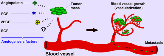
Angiogenesis is an intricate process in the human body in which endothelial cells proliferate, migrate and remodel themselves from from pre-existing blood vessels, formed during early vasculogenesis. It is involved in a variety of healthy physiological functions such as embryonic development, wound healing, and collateral formation for improved organ perfusion [2]. However, it is also one of the hallmarks of metastatic cancer: the process of angiogenesis provides the tumor with the needed oxygen and nutrients to grow and metastasize to other parts of the body. In other words, the formation of these new blood vessels serves as the principle route for the tumor cells to exit the primary tumor site and enter circulation [3]. Figure 1 from [2] gives a concise picture of the process of tumor angiogenesis:
Figure 1. Depiction of the Tumor Angiogenesis Process.
Recently, much biomedical research has gone into creating effective anti-angiogenesic inhibitors. As a result, a plethora of anti-angiogenic agents such as Avastin, Nexavar, and Zaltrap have been developed. The effectiveness of these agents have been analyzed to be mediocre, at best, and it has been shown that pharmacologic anti-angiogenic protocols which arrest tumor progression is often not enough to eradicate tumors [2]. As such, physicians are now starting to use anti-angiogenic inhibitors in conjunction with other therapies such as immunotherapy or chemotherapy [4]. A recent mathematical modeling paper showed the effectiveness of anti-angiogenic drugs when used in combination with immunotherapy, displaying through a bifurcation analysis how the former supplements the latter, leading to earlier tumor remission [1]. However, the paper does not analyze when this combination treatment should be used in the clinic, i.e., when used with immunotherapy, when does the anti-angiogenic treatment cause more harm than benefits? Through optimal control analysis, this is the question we attempt to answer here. The paper is organized as follows: first, the mathematical model proposed in [1] is summarized along with its nondimensionalization. Then, an analytic optimal control analysis is performed, giving optimality conditions for the administration of immunotherapy and anti-angiogenic drugs. Then, parameter values determined in [1] are provided and used to perform numerical simulations for a control patient, and for patients with different side effects for each treatment. Finally, a brief conclusion is given for this paper.
2. Model Description
The author analyzes the model originally constructed in [1]. This model considers dynamics among host cells \((x)\), cancer cells \((y)\), endothelial cells \((z)\), effector cells \((v)\), and anti-angiogenesis \((w)\). The model is reproduced below:
\begin{eqnarray*}&&\frac{dX}{dt}= \alpha_1X\Big(1-\frac{X}{K_1}\Big)-Q_1XY,\\
&&\frac{dY}{dt}= \alpha_2Y\Big(1-\frac{Y}{K_2+BZ}\Big)-Q_2XY-Q_3YV+P_2YZ,\\
&&\frac{dZ}{dt}= CY+\alpha_3Z\Big(1-\frac{Z}{K_3}\Big)-\frac{P_3ZW}{A_3+Z},\\
&&\frac{dV}{dt} = S_1+RY-D_4V,\\
&&\frac{dW}{dt} = S_2-\frac{P_5ZW}{A_3+Z}-D_5W.\end{eqnarray*}
In this model, \(\alpha_i\) represent the natural growth rate of the populations, \(K_i\) represent the carrying capacities, and \(Q_i\) represent intracellular competition. B represents the portion of the endothelial cell population responsible for tumor angiogenesis, \(P_2\) is the promotion coefficient of endothelial cells to cancer cells, C is the rate of production of cancer cells due to endothelial cells, R represents the rate of recruitment of effector cells due to cancer cells, \(D_{4,5}\) are the washout rates of effector cells and the anti-angiogenic agent, and the \(\frac{P_iZW}{A_3+Z}\) are the functions of Holling II functional response, capturing the saturating effects of the anti-angiogenic response.
To further clarify the dependence of the system on parameters, and to
improve the performance of numerical methods, the system is non-dimensionalized as follows. The nondimensionalzed state variables are \(x=\frac{X}{K_1}\), \(y=\frac{Y}{K_2}\), \(z=\frac{Z}{K_3}\), \(v=V\), \(w=W\) and the corresponding parameters are \(q_1=Q_1K_2\), \(\gamma=\frac{BK_3}{K_2}\), \(q_2=Q_2K_1\), \(q_3=Q_3\), \(p_2=P_2K_3\), \(\beta=\frac{CK_2}{K_3}\), \(p_3=\frac{P_3}{K_3}\), \(a_3=\frac{A_3}{K_3}\), \(d_i=D_i\), \(r=K_2R\), \(p_5=P_5\). Then, the nondimensionalized system is given by:
\begin{eqnarray*}
\frac{dx}{dt} &=& \alpha_1x(1-x)-q_1xy,\\
\frac{dy}{dt} &=& \alpha_2y\Big(1-\frac{y}{1+\gamma z}\Big)-q_2xy-q_3yv+p_2yz,\\
\frac{dz}{dt} &=& \beta y+\alpha_3z(1-z)-\frac{p_3zw}{a_3+z},\\
\frac{dv}{dt} &=& S_1+ry-d_4v,\\
\frac{dw}{dt} &=& S_2-\frac{p_5zw}{a_3+z}-d_5w.\end{eqnarray*}
3. Optimal control analysis
Here, we formulate the problem of constructing the most effective treatment regimen as an optimal control problem. To do this, we first modify the model slightly to incorporate the controls by adding “scaling control” factors to the \(S_1\) and \(S_2\) therapy administration terms:
\begin{eqnarray*}\frac{dx}{dt} &=& \alpha_1x(1-x)-q_1xy,\\
\frac{dy}{dt} &=& \alpha_2y\Big(1-\frac{y}{1+\gamma z}\Big)-q_2xy-q_3yv+p_2yz,\end{eqnarray*}
\begin{eqnarray*}\frac{dz}{dt} &=& \beta y+\alpha_3z(1-z)-\frac{p_3zw}{a_3+z},\\
\frac{dv}{dt} &=& u_{imm}(t)S_1+ry-d_4v,\\
\frac{dw}{dt} &=& v_{ang}(t)S_2-\frac{p_5zw}{a_3+z}-d_5w.\end{eqnarray*}
We want to maximize the number of host and effector cells while minimizing the number of cancer cells and amount of anti-angiogenic inhibitor and immunotherapy prescribed over a fixed therapy interval \([0,T].\)
We choose as our control class piecewise continuous functions defined for all \(t\) such that \(0 \leq u_{imm}(t) \leq 1\) where \(u_{imm}(t)= 1\) represents maximal chemotherapy and \(u_{imm}(t) = 0\) represents no chemotherapy. Similarly, \(v_{ang}(t) = 0\) represents no anti-angiogeneic inhibitors and \(v_{ang}(t) = 1\) represents maximal anti-angiogenic drug. Thus, we depict the class of admissible controls as:
\begin{equation*}
U(t) = u_{imm}(t), v_{ang}(t)\;\; \text{piecewise continuous such that}\;\; 0 \leq u_{imm}(t), v_{ang}(t) \leq 1, \forall t \in [0, T]
\end{equation*}
Now, we define my objective functional and optimal control problem. For a fixed therapy horizon \([0,T],\) maximize the objective functional:
\begin{equation}
J(u,v) = \int_{0}^{T} \alpha v+\theta x-\frac{1}{2}b_1u_{imm}^2-\frac{1}{2}b_2v_{ang}^2-\psi y dt
\end{equation}
(1)
over all Lebesgue-measurable functions \(u:[0,T] \rightarrow [0,u_{max}]\) and \(v:[0,T] \rightarrow [0,v_{max}]\) subject to the above ODE dynamics and initial conditions of \(x(0) = 0.8, y(0) = 0.0006, z(0) = v(0) = w(0) = 0.\)
3.1. Existence of optimal control
The existence of an optimal control for the state system is analyzed using the theory developed in [5]. The boundedness of solutions of the system for finite time is needed to obtain existence and uniqueness of an optimal control. Using \(y(t)< K_2\), the carrying capacity of the cancer cell population, upper bounds on the solutions of the state system are determined.
\begin{eqnarray*}
\frac{d\bar{x}}{dt} &=& \alpha_1\bar{x},\\
\frac{d\bar{y}}{dt} &=& \alpha_2\bar{y}+p_2\bar{z}K_2,\\
\frac{d\bar{z}}{dt} &=& \beta \bar{y}+\alpha_3\bar{z},\\
\frac{d\bar{v}}{dt} &=& S_1+r\bar{y},\\
\frac{d\bar{w}}{dt} &=& S_2.\end{eqnarray*}
The supersolutions \(\bar{x},\bar{y},\bar{z},\bar{v},\bar{w}\) of the above system are bounded on a finite time interval. The system can also be written, where \('=\frac{d}{dt}\), as
Since this is a linear system in finite time with bounded coefficients, the supersolutions \(\bar{x},\bar{y},\bar{z},\bar{v},\bar{w}\) are uniformly bounded. Using that the solution to each state
equation is bounded, we now prove the existence of an optimal control.
Theorem 1. There exists optimal controls \(u_{imm}\) and \(v_{ang}\) that maximizes the objective functional J(u,v) if the following conditions are met:
The class of all initial conditions with controls \(u_{imm}\) and \(v_{ang}\) such that \(u_{imm}\) and \(v_{ang}\) are Lebesgue integrable functions on [0,T] with values in the admissible control set along with each state equation being satisfied is not empty
The admissible control set is closed and convex
The right hand side of the state system is continuous, is bounded above by a sum of the bounded control and the state, and can be written as a linear function of
\(u_{imm}\) and \(v_{ang}\) with coefficients depending on time and the state variables
The integrand of the functional is concave on the admissible control set and is bounded above by \(c_3 – c_2|u_{imm}|^\theta – c_1|v_{ang}|^\phi\), where \(c_1, c_2 > 0\), and \(\theta, \phi > 1\).
Proof.
First, from a result in [6], since our state system has bounded coefficients and any solutions are bounded on the finite time interval, we obtain
the existence of the solution of the state system. Second, the admissible control set is closed and convex, by definition. For the third condition, the right hand side of the state system is continuous since each term with a denominator is nonzero. Moreover, the
system is bilinear in the controls and can be rewritten as
where \(C_1\) depends on the coefficients of the system. Also, note that the integrand of J(u,v) is concave on the admissible control set. The existence of optimal control follows from the fact that \(\alpha v+\theta x-\frac{1}{2}b_1u_{imm}^2-\frac{1}{2}b_2v_{ang}^2-\psi y \leq c_3 – c_2|u_{imm}|^\theta – c_1|v_{ang}|^\phi\), where \(c_1, c_2 > 0\), and \(\theta, \phi > 1\) since \(y(t) \leq K_2\).
3.2. Characterization of optimal control
Now, we characterize the optimal control pair \((u_{imm},v_{ang})\). Conditions for optimality are determined by a version of the Pontgaryin maximum principle. The existence of an optimal control pair is ensured by the compactness of the control and state spaces, in addition to the convexity of the problem. First, we define the Lagrangian associated with \(J(u,v)\) and our ODE model as follows:
\(L = \alpha v+\theta x-\frac{1}{2}b_1u_{imm}^2-\frac{1}{2}b_2v_{ang}^2-\psi y + \lambda_1(\alpha_1x(1-x)-q_1xy) + \lambda_2\Big(\alpha_2y\Big(1-\frac{y}{1+\gamma z}\Big)-q_2xy-q_3yv+p_2yz\Big) + \lambda_3\Big(\beta y+\alpha_3z(1-z)-\frac{p_3zw}{a_3+z}\Big) + \lambda_4(u_{imm}(t)S_1+ry-d_4v) + \lambda_5\Big(v_{ang}(t)S_2-\frac{p_5zw}{a_3+z}-d_5w\Big) + j_1(t)(u_{imm})+j_2(t)(1-u_{imm})+k_1(t)v_{ang}+k_2(t)(1-v_{ang}).\)
Note that the last \(j\) and \(k\) terms have been added in to serve as penalty multipliers for non-optimal controls:
\begin{equation*}
j_1(t)u_{imm} = j_2(t)(1-u_{imm}) = k_1(t)v_{ang} = k_2(t)(1-v_{ang}) = 0
\end{equation*}
for the optimal controls \((u_{imm}^*, v_{ang}^*)\).
Theorem 2.Given optimal controls \(u_{imm}^*\) and \(v_{ang}^*\) and solutions of the corresponding state system, there exist adjoint variables \(\lambda_i\) for i = 1, 2, 3, 4, 5 satisfying:
\begin{eqnarray*}
\frac{d\lambda_1}{dt} = -\frac{\partial L}{\partial x} &=& -[\theta+ \lambda_1(\alpha_1(1-2x)-q_1y)-\lambda_2yq_2],\\
\frac{d\lambda_2}{dt} = -\frac{\partial L}{\partial y} &=& -\Big[-\psi -\lambda_1(q_1x) – \lambda_2\Big(\alpha_2\Big(1-\frac{2y}{1+\gamma z}\Big)-q_2x-q_3v+zp_2\Big) + \lambda_3 \beta + \lambda_4 r\Big],\\
\frac{d\lambda_3}{dt} = -\frac{\partial L}{\partial z} &=& -\Big[\lambda_2\Big(\frac{\alpha_2y^2\gamma}{(\gamma z+1)^2}+yp_2\Big)+\lambda_3\Big(\alpha_3(1-2z)-\frac{a_3p_3w}{(a_3+z)^2}\Big)+\lambda_5\Big(-\frac{a_3p_5w}{(a_3+z)^2}\Big)\Big],\end{eqnarray*}
\begin{eqnarray*}
\frac{d\lambda_4}{dt} &=& -\frac{\partial L}{\partial v} = -[\alpha – \lambda_2q_3y – \lambda_4d_4],\\
\frac{d\lambda_5}{dt} &=& -\frac{\partial L}{\partial w} = -\Big[\lambda_3\Big(-\frac{p_3z}{a_3+z}\Big)-\lambda_5\Big(\frac{p_5z}{a_3+z}+d_5\Big)\Big],\end{eqnarray*}
where \(\lambda_i(T)=0\) for i=1, 2, 3, 4, 5 by the PMP transversality condition. Furthermore, from the optimality condition, \(u_{imm}^*\) is given by:
Proof.
Since the state variables are bounded, the maximum principle guarantees existence of the adjoint variables, as described above. The Lagrangian was maximized with respect to the variables in the optimal control pair by differentiating L with respect to \(u_{imm}\) and \(v_{ang}\). By doing this, we get the following:
And thus the representation of \(v_{ang}^*\) is \(\frac{\lambda_5S_2}{b_2}\).
Then, by using the bounds \(0 \leq u_{imm} \leq 1\) and \(0 \leq v_{ang} \leq 1\), we obtain the explicit control profiles given in Equations 2 and 6.
Since both state and adjoint solutions are \(L^\infty\)-bounded, the right side of the adjoint and state equations are Lipschitz for those solutions. This furthermore ensures that the solution of the optimality system is unique, given that the final time is not very large. A rigorous proof of such an argument can be found in [7] and [8]. Obviously, the uniqueness of the solutions for the optimality system implies uniqueness of the optimal control pair. Now, we have an explicit formulation for optimal controls, coupling the adjoint with the state equations and the initial and transversality conditions give the following optimality system:
\begin{eqnarray*}
\frac{dx}{dt} &=& \alpha_1x(1-x)-q_1xy,\\
\frac{dy}{dt} &=& \alpha_2y\Big(1-\frac{y}{1+\gamma z}\Big)-q_2xy-q_3yv+p_2yz,\\
\frac{dz}{dt} &=& \beta y+\alpha_3z(1-z)-\frac{p_3zw}{a_3+z},\\
\frac{dv}{dt}& =& min\Big(max\Big(0,\frac{\lambda_4S_1}{b_1}\Big),1\Big)S_1+ry-d_4v,\\
\frac{dw}{dt} &=& min\Big(max\Big(0,\frac{\lambda_5S_2}{b_2}\Big),1\Big)S_2-\frac{p_5zw}{a_3+z}-d_5w,\\
\frac{d\lambda_1}{dt} &=& -\frac{\partial L}{\partial x} = -[\theta+ \lambda_1(\alpha_1(1-2x)-q_1y)-\lambda_2yq_2],\\
\frac{d\lambda_2}{dt} &=& -\frac{\partial L}{\partial y} = -\Big[-\psi -\lambda_1(q_1x) – \lambda_2\Big(\alpha_2\Big(1-\frac{2y}{1+\gamma z}\Big)-q_2x-q_3v+zp_2\Big) + \lambda_3 \beta + \lambda_4 r\Big],\\
\frac{d\lambda_3}{dt} &=& -\frac{\partial L}{\partial z} = -\Big[\lambda_2\Big(\frac{\alpha_2y^2\gamma}{(\gamma z+1)^2}+yp_2\Big)+\lambda_3\Big(\alpha_3(1-2z)-\frac{a_3p_3w}{(a_3+z)^2}\Big)+\lambda_5\Big(-\frac{a_3p_5w}{(a_3+z)^2}\Big)\Big],\\
\frac{d\lambda_4}{dt} &=& -\frac{\partial L}{\partial v} = -[\alpha – \lambda_2q_3y – \lambda_4d_4],\\
\frac{d\lambda_5}{dt} &=& -\frac{\partial L}{\partial w} = -\Big[\lambda_3\Big(-\frac{p_3z}{a_3+z}\Big)-\lambda_5\Big(\frac{p_5z}{a_3+z}+d_5\Big)\Big].
\end{eqnarray*}
4. Parameter values
We obtain the parameter values given in Table 1 to be used in the numerical optimal control and simulation experiments from [1].
Table 1. Parameters Used in Numerical Simulations.
Parameter
Estimated Value
\(\alpha_1\)
6800
\(\alpha_2\)
0.01
\(\alpha_3\)
0.002
\(r\)
0.002
\(p_5\)
0.032
\(q_1\)
0.0072
\(q_2\)
0.00072
\(\beta\)
0.004
\(d_4\)
0.0132
\(d_5\)
0.136
\(q_3\)
0.01
\(p_3\)
1.8
\(p_2\)
0.002
\(a_3\)
0.49
\(\gamma\)
0.15
\(S_1\)
0.017
\(S_2\)
0.07
5. Numerical simulations
Several numerical simulations have been performed using the Python GEKKO optimization suite for different hypothetical patients. Though the model parameters remained constant for all patients, the weights in the objective functional were modified. All parameter values used can be found in Table 1; the initial values used were \(x = 0.8\), \(y = 0.0006\), \(z = v = w = 0\).
5.1. Control simulations
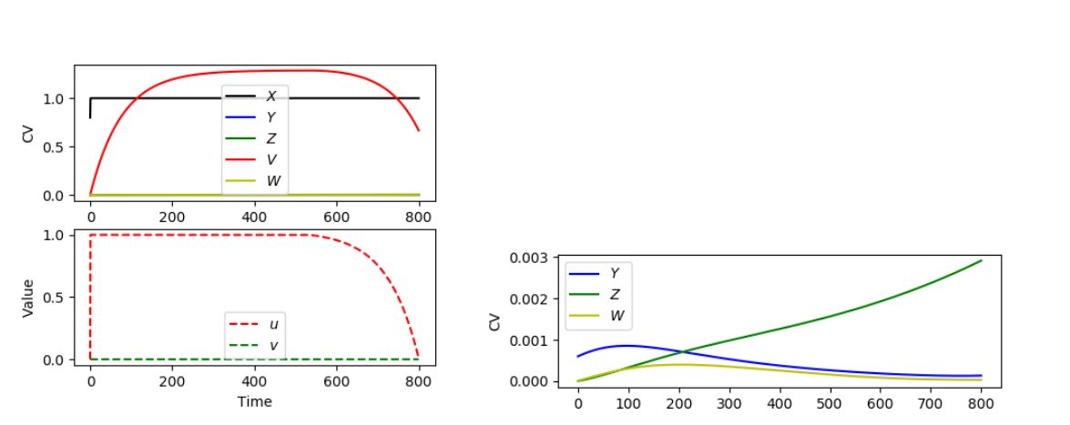
The first simulation run, shown in Figure 2, was the control simulation. In this simulation, the following values were used for the weighting parameters of the objective functional: \(\alpha = 1.2\), \(b_1 = 1.5\), \(b_2 = 1.5\), \(\theta = 1.3\), and \(\psi = 3.0\).
Figure 2. Numerical Optimal Control and Treatment Simulation Results – Control Case.
The figure on the left represents the overall dynamics of the system along with the optimal control profile; the right figure zooms in on the anti-angiogenesis and cancer and endothelial cells. As we can see, in this case, optimal control profile indicates that virtually no anti-angiogenic therapy should be used, while the immunotherapy should be used at full potential for the first \(\approx 600\) days, before quickly tapering off to 0 by the 800th day. We note that the effector and host cell population are at healthy levels, with the endothelial population rising and the tumor population reaching zero.
5.2. Patient-specific side effect simulations
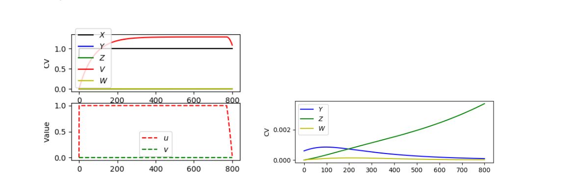
The second simulation run was one in which there was an especially low immunotherapy side effect. The same weighting values as the control were used, but the \(b_1\) parameter was reduced to 0.5. The results can be seen below in Figure 3:
Figure 3. Numerical Optimal Control and Treatment Simulation Results – Low Immunotherapy Side Effect Case.
Here, we see a similar optimal control profile to the control, but the immunotherapy treatment was used for a much longer time (until \(\approx 780\) days), before the treatment was stopped much more abruptly; no anti-angiogenic treatment was detected at all in this case. The final dynamics observed healthy levels of effector and host cells, with growing levels of endothelial cells and tumor remission.
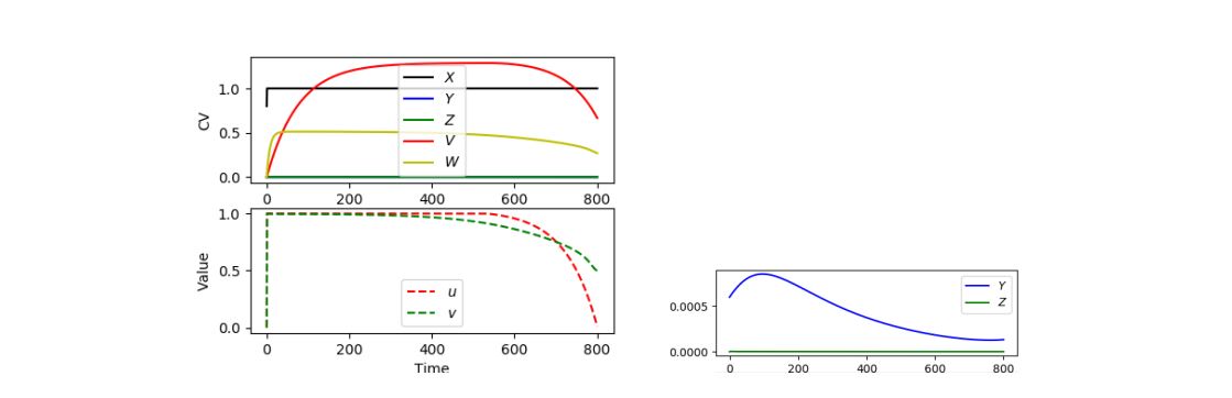
Next, a simulation for extremely low anti-angiogenic side effects was run. Control weighting parameters were used, but the \(b_2\) parameter was changed to 0.005. The results are seen in Figure 4 below:
Figure 4. Numerical Optimal Control and Treatment Simulation Results – Low Anti-Angiogenic Side Effect Case.
This is the first case in which we notice a strong presence of anti-angiogenic use. Note, however, that the weightage term used for the side effects of anti-angiogenic drugs is extreme, and not typical of most patients (unless additional medications are given to offset the side effects). Here, we see that it is recommended that both treatments are initially given at full potential. At \(\approx 300\) days, both treatments begin tapering off, with the anti-angiogenic treatment tapering off more slowly. By the day 800, the immunotherapy treatment has stopped, while the anti-angiogenic treatment is still prescribed at half of full capacity. Note that here, the effector and host cell populations are at healthy levels, though the endothelial cells are at zero, and there is a very small non-zero tumor value at 800 days.
Finally, a simulation was run for extremely high immunotherapy side effects. The same parameters as the control were used, but the \(b_1\) term was changed to 10. The results are shown in Figure 5:
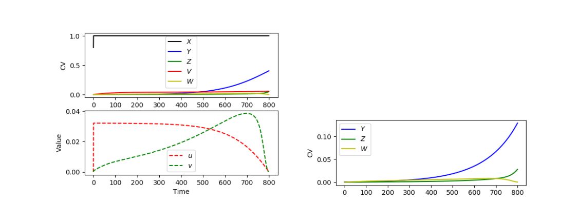
Figure 5. Numerical Optimal Control and Treatment Simulation Results – High Immunotherapy Side Effect Case.
This is also medically not typical unless the patient suffers from the rare side effects of pneumonitis, hepatitis, colitis, severe hormonal/gland problems, or severe brain inflammation such as neuropathy, meningitis, or encephalitis. In this case, we note that both drugs are given at very low frequencies (up to 4% of their potentials). The immunotherapy is given at about 0.035 for the first \(\approx\) 450 days, before tapering off to 0 by day 800. The anti-angiogenic drug steadily rises to a value of 0.04 by day 700, after which it plummets to 0 by the day 800. Note here that, though the host cell population is healthy, the cancerous cell are rapidly growing; the endothelial cells show more modest growth.
Thus, it can be concluded that, as seen in [1], immunotherapy is typically the most effective at causing tumor remission. In the cases that the optimal profile included anti-angiogenic drugs, we note that the cancer cell population was not completely eradicated. We also notice that anti-angiogenic drugs are only included in the optimal profile if the side effects of them are almost none, or if the side effects of immunotherapy are very high.
Therefore, as stated in [1], though it may be the case that the anti-angiogenic drugs can aid immunotherapy treatment plans, in most cases, this is not part of the optimal treatment profile.
6. Conclusion
In this paper, a detailed optimal control analysis was performed on the model developed in [1] on a combination immunotherapy-anti-angiogenic drug therapy treatment regimen. An analytic characterization of optimal control protocols was given, along with comments on the existence and uniqueness of such profiles. Numerical simulations were performed for a variety of patients, using different weighting terms in the objective functional. It was found that, except for the most extreme cases, the use of anti-angiogenic inhibitors was not justified. The author hopes that this work will help inspire further research into the consideration of more effective, synergetic combination therapies involving anti-angiogenic inhibitors and perhaps into the further development of more effective anti-angiogenic drugs.
Acknowledgments
The author wishes to express his profound gratitude to the reviewers for their useful comments on the manuscript.
Author Contributions
All authors contributed equally to the writing of this paper. All authors read and approved the final manuscript.
Competing Interests
The author(s) do not have any competing interests in the manuscript.
References
Shi, X., He, X., & Ou, X. (2015, December). A mathematical model and analysis of the anti-angiogenic and tumor immunotherapy. In 2015 4th International Conference on Computer Science and Network Technology (ICCSNT) (Vol. 1, pp. 1549-1553). IEEE. [Google Scholor]
Rajabi, M., & Mousa, S. A. (2017). The role of angiogenesis in cancer treatment. Biomedicines, 5(2), 34. [Google Scholor]
Zetter, B. R. (1998). Angiogenesis and tumor metastasis. Annual review of medicine, 49(1), 407-424. [Google Scholor]
Ma, J., & Waxman, D. J. (2008). Combination of antiangiogenesis with chemotherapy for more effective cancer treatment. Molecular cancer therapeutics, 7(12), 3670-3684. [Google Scholor]
Fleming, W. H., & Rishel, R. W. (2012). Deterministic and stochastic optimal control (Vol. 1). Springer Science & Business Media. [Google Scholor]
Lukes, D. L. (1982). Differential equations: classical to controlled. Elsevier.[Google Scholor]
Burden, T. N., Ernstberger, J., & Fister, K. R. (2004). Optimal control applied to immunotherapy. Discrete and Continuous Dynamical Systems Series B, 4(1), 135-146. [Google Scholor]
Fister, K. R., Lenhart, S. & McNally, J. S. (1998). Optimizing chemotherapy in an HIV model. Electronic Journal of Differential Equations, 1998(32), 1-12. [Google Scholor]