This paper investigates the squeezing flow of an electrically conducting magnetohydrodynamic Casson nanofluid between two parallel plates embedded in a porous medium using differential transformation and variation of parameter methods. The accuracies of the approximate analytical methods for the small and large values of squeezing and separation numbers are investigated and established. Good agreements are established between the results of the approximate analytical methods are compared with the results numerical method using fourth-fifth order Runge-KuttaFehlberg method. However, the results of variation of parameter methods show better agreement with the results of numerical method than the results of differential transformation method. Thereafter, the developed approximate analytical solutions are used to investigate the effects of pertinent flow parameters on the squeezing phenomena of the nanofluids between the two moving parallel plates. The results established that the squeezing number and magnetic field parameters decrease as the flow velocity increases when the plates were coming together. Also, the velocity of the nanofluids further decreases as the magnetic field parameter increases when the plates move apart. However, the velocity is found to be directly proportional to the nanoparticle concentration during the squeezing flow i.e. when the plates are coming together and an inverse variation between the velocity and nanoparticle concentration is recorded when the plates are moving apart. As increased physical insights into the flow phenomena are provided, it is hope that this study will enhance the understanding the phenomena of squeezing flow in various applications such as power transmission, polymer processing and hydraulic lifts.
Keywords: Casson fluid, squeezing flow, nanofluid, magnetic field, differential transformation method, variation of parameter method.
1. Introduction
The various applications of fluid flow between two parallel surfaces require to more intensive research. These applications are evident in foodstuff processing, reactor fluidization, moving pistons, chocolate fillers, hydraulic lifts, electric motors, flow inside syringes and nasogastric tubes, compression, and injection, power transmission squeezed film, polymers processing etc. In such fluid flow applications and processes, analysis of momentum equation is very essential. The basic and pioneer study on squeezing flows under lubrication assumption was given by Stefan [1]. Thereafter, there have been increasing research interests and many scientific studies on these types of flow. In a past work over few decades, Reynolds [2] analyzed the squeezing flow between elliptic plates while Archibald [3] investigated the same problem for rectangular plates. The earlier studies on squeezing flows were based on Reynolds equation which its insufficiency for some cases has been shown by Jackson [4] and Usha and Sridharan [5]. Moreover, the nonlinear behaviours of the flow phenomena have attracted several attempts and renewed research interests aiming at properly analyzing and understanding the squeezing flows [6, 7, 8, 9, 10, 11, 12, 13, 14, 15, 16, 17, 18, 19, 20, 21, 22, 23, 24, 25, 26, 27, 28, 29, 30, 31, 32, 33, 34, 35, 36].
Casson fluid is a non-Newtonian fluid first invented by Casson in 1959 [37, 38]. It is a shear thinning liquid which is assumed to have an infinite viscosity at zero rate of shear, a yield stress below which no flow occurs, and a zero viscosity at an infinite rate of shear [39]. It is based on the structure of liquid phase and interactive behaviour of solid of a two-phase suspension. It is able to capture complex rheological properties of a fluid, unlike other simplified models like the power law [40] and second, third or fourth-grade models [41]. The non-linear Casson’s constitutive equation has been found to describe accurately the flow curves of suspensions of pigments in lithographic varnishes used for preparation of printing inks. In particular, the Casson fluid model describes the flow characteristics of blood more accurately at low shear rates and when it flows through small blood vessels [42]. So, human blood can also be treated as a Casson fluid in the presence of several substances such as fibrinogen, globulin in aqueous base plasma, protein, and human red blood cells. Some famous examples of the Casson fluid include jelly, tomato sauce, honey, soup, concentrated fruit juices etc. Concentrated fluids like sauces, honey, juices, blood, and printing inks can be well described using the Casson model. Many researchers [43, 44, 45, 46, 47, 48, 49, 50, 51, 52] studied the Casson fluid under different boundary conditions. Some find the solutions by using either approximate methods or numerical schemes and some find its exact analytical solutions. The solutions when the Casson fluids are in free convection flow with constant wall temperature are also determined. On the other hand, the flow of the Casson fluid in the presence of heat transfer is also an important research area. Therefore, Khalid et al. [53] focused on the unsteady flow of a Casson fluid past an oscillating vertical plate with constant wall temperature under the non-slip conditions. Application of Casson fluid for flow between two rotating cylinders is performed in [54]. The effect of magnetohydrodynamic (MHD) Casson fluid flow in a lateral direction past linear stretching sheet was explained by Nadeem et al. [55].
To the best of the authors’ knowledge, a comparative study on squeezing flow of an electrically conducting Casson nanofluid between two parallel plates embedded in porous medium under the influence of magnetic field using differential transformation and variation of parameter methods has not been carried out in literature. Therefore, in this paper, a comparative study and analytical investigations are presented using differential transformation and variation of parameter methods to analyze the magnetohydrodynamic squeezing flow of Casson nanofluid between two parallel plates embedded in a porous medium. The developed analytical solutions are used to study the effects of various parameters on the squeezing flow between two parallel plates.
2. Problem Formulation
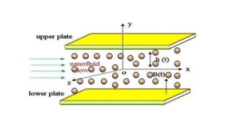
As depicted in Figure 1, the flow of a Casson nanofluid between two parallel plates placed at time-variant distance and under the influence of magnetic field is considered in this study. Assuming that the flow of the nanofluid is laminar, stable, incompressible, isothermal, non-reacting chemically, the nano-particles and base fluid are in thermal equilibrium and the physical properties are constant. The fluid conducts electrical energy as it flows unsteadily under magnetic force field. The fluid structure is everywhere in thermodynamic equilibrium and the plate is maintained at constant temperature.
Figure 1. Model diagram of MHD squeezing flow of nanofluid between two parallel plates embedded in a porous medium.
Based on the rheological equation for an isotropic and incompressible Casson fluid as reported by Casson [37, 38], we have
The physical properties of the copper nanoparticles, pure water and kerosene as the base fluids are shown in Table 1.
Table 1. Physical properties of copper nanoparticles, water and kerosene.
Density (kg/m3)
Dynamic viscosity (kg/ms)
Pure water
997.1
0.000891
Kerosene
783.0
0.001640
Copper
8933.0
–
3. Analysis of the differential equation using differential transform method
Following the introduction of differential transformation method (DTM) by Zhou [56], the applications of DTM to both linear and non-linear differential and system of differential equation have fast gained ground or appeared in many engineering and scientific research. The potentiality of the method is displayed in the provisions of symbolic or analytical solutions to both linear and non-linear integral and differential equations without linearization, discretization or perturbation. DTM is capable of greatly reducing the size of computational work while still accurately providing the series solution with fast convergence rate. The basic definitions and the operational properties of the method are as follows:
If \(u(t)\) is analytic in the domain \(T,\) then the function \(u(t)\) will be differentiated continuously with respect to time \(t.\)
\begin{equation}\label{eq11}
\frac{d^{p} u(t)}{dt^{p} } =\varphi (t,p) \text{ for all } t\in T
\end{equation}
(14)
for \(t=t_{i} \), then \(\varphi (t,p)=\varphi (t_{i} ,p)\) , where \(p\) belongs to the set of non-negative integers, denoted as the \(p\)-domain. We can therefore write Equation (14) as
where Equation (16) is the inverse of \(U(k)\). The symbol \(`D’\) denoting the differential transformation process and combining (15) and (16), we have
On solving the above Equation (23) and Equation (24), different values for \(k_{1}\) and \(k_{2}\) for respective different values of \(Re\) and \(\alpha\) were obtained.
For the purpose of comparison, the second-order derivatives of \(f(1)\) at the wall (which represent the skin friction) is developed as
The linear terms are decomposed into \(L + R,\) with \(L\) taken as the highest order derivative which is easily invertible and R as the remainder of the linear operator of order less than \(L.\) where \(g\) is the system input or the source term and \(u\) is the system output, \(Nu\) represents the nonlinear terms.
The VPM provides the general iterative scheme for Equation (26) as:
\(m\) is the order of the given differential equation, \(k_{i}\) is are the unknown constants that can be determined by initial/boundary conditions and \(\lambda (\eta ,\xi )\) is the multiplier that reduces the order of the integration and can be determined with the help of Wronskian technique.
Here, \(k_{1}\), \(k_{2}\), \(k_{3}\), and \(k_{4}\) are constants obtained by taking the highest order linear term of Equation (12) and integrating it four times to get the final form of the scheme.
The above equation can also be written as
From the boundary conditions in Equation (13)
\[f(0)=0,\quad f”(0)=0.\]
Using the above statement and inserting the boundary conditions of Equation (13) into Equation (31), we have
Tables 3,4,5 show the comparisons of results of DTM and VPM with the results of the numerical method (NM) for different values of permeation Reynolds and Hartmann numbers. From the results, it shows that the results of VPM agree excellently well with the results of numerical method. Although, the results of DTM also agrees very well with the results of the numerical methods, better agreements are established between the results of VPM and NM.
Table 3. Comparison of results of flow for large squeezing number in the absence of magnetic field.
f
Squeezing S= 101,
M=0,
1/Da=0
\(\eta\)
NM
DTM
VPM
0.0
0.00000
0.00000
0.00000
0.1
0.16377
0.16376
0.16377
0.2
0.32193
0.32194
0.32193
0.3
0.46995
0.46992
0.46995
0.4
0.60424
0.60422
0.60424
0.5
0.72190
0.72191
0.72190
0.6
0.82063
0.82063
0.82063
0.7
0.89871
0.89874
0.89971
0.8
0.95498
0.95496
0.95498
0.9
0.98878
0.98875
0.98878
1.0
1.00000
1.00000
1.00000
Table 4. Comparison of results of skin friction for large separation number under the influence of magnetic field.
$$f”(1)$$
S
M
NM
DTM
VPM
12.957
6.445
-4.78
-4.78
-4.78
18.638
6.103
-4.07
-4.07
-4.07
25.747
7.151
-4.11
-4.11
-4.11
41.818
11.419
-5.10
-5.10
-5.10
50.460
9.964
-4.16
-4.16
-4.16
62.485
11.077
-4.17
-4.17
-4.17
76.326
12.233
-4.18
-4.18
-4.18
Table 5. Comparison of results for small squeezing number in the absence of magnetic field.
f
Squeezing S= 0.5,
M=0,
1/Da=0
f Squeezing S= 1.5,
M=0,
1/Da=0
\(\eta\)
NM
DTM
VPM
\(\eta\)
NM DTM
VPM
0.0
0.00000
0.00000
0.00000
0.00000
0.00000
0.00000
0.2
0.31707
0.31705
0.31707
0.31609
0.31607
0.31609
0.4
0.59972
0.59971
0.59971
0.59818
0.59820
0.59818
0.6
0.81886
0.81884
0.81884
0.81747
0.81743
0.81747
0.8
0.95526
0.95525
0.95525
0.95430
0.95432
0.95430
1.0
1.00000
1.00000
1.00000
1.00000
1.00000
1.00000
Apart from the fact that Tables 3,4,5 show the comparison of results, they also depict the effects of various parameters on the squeezing flow. It is shown that the velocity of the flow increases as the fluid moves away from the plates. The skin friction coefficient decreases as the separation number and the Magnetic field increases when the plates separate apart while skin friction coefficient decreases as the squeezing number and the magnetic field increase when the plates come together. The flow velocity of the nanofluid decreases as the magnetic parameter increases. The flow response to the presence of magnetic field is due to the Lorentz force created by the magnetic field which slows fluid motion at boundary layer during the squeezing flow i.e. when the plates are coming together. It should be noted that during the squeezing flow, especially when the plates are very close to each other, then the situation together with retarding Lorentz force creates adverse pressure gradient. Whenever such forces act over a long time then there might be a point of separation and back flow occurs. The flow velocity of the nanofluids further decreases as the magnetic field parameter increases when the plates move apart. The flow behaviour when the plates move apart is because a vacant space occurs and in order not to violate the law of conservation of mass, the fluid in that region moves with high velocity and consequently, an accelerated flow is observed.
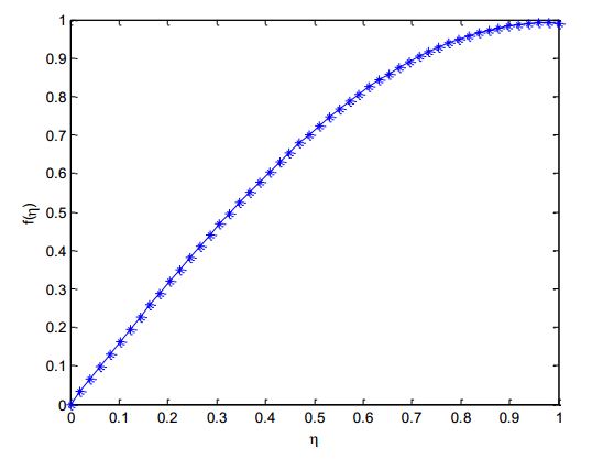
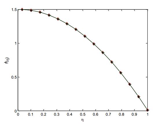
For the nanoparticle parameter value of 0.15 i.e. \(\mathrm{\phi}\) = 0.15, Figures 2 and 3 depict the pattern of the flow behavior of the fluid. The figures show that the decrease in the axial velocity of the fluid near the wall region causes an increase in velocity gradient at the wall region. Also, because of the conservativeness of the mass flow rate, the decrease in the fluid velocity near the wall region is compensated by the increasing fluid velocity near the central region.
Figure 2. Figure 2a Variation of \(f(\eta)\) with the flow length.Figure 3. Variation of \(f’(\eta)\) with the flow length.Figure 4. Effects of magnetic number on the velocity of the fluid.Figure 5. Effects of Darcy number on the velocity.Figure 6. Effects of Squeezing number on the velocity.Figure 7. Effects of nanoparticle fraction on the velocity.Figure 8. Effects of Casson fluid parameter on the velocity.
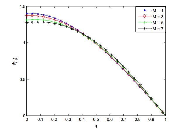
Figure 3 which shows the effect of increasing magnetic number or Hartmann parameter (M), it is observed that at increasing values of \(M\) the velocity decreases the velocity decreases in the range of \(0\mathrm{\le}\eta\mathrm{\le} 0.5\) and then increases in the range \(0.5 \mathrm< \eta\mathrm\le 1.\) The flow response to the presence of magnetic field is due to the Lorentz force created by the magnetic field which slows fluid motion at boundary layer during the squeezing flow i.e. when the plates are coming together. It should be noted that during the squeezing flow, especially when the plates are very close to each other, then the situation together with retarding Lorentz force creates adverse pressure gradient. Whenever such forces act over a long time then there might be a point of separation and back flow occurs. The flow velocity of the nanofluids further decreases as the magnetic field parameter increases when the plates move apart. The flow behaviour when the plates move apart is because a vacant space occurs and in order not to violate the law of conservation of mass, the fluid in that region moves with high velocity and consequently, an accelerated flow is observed.
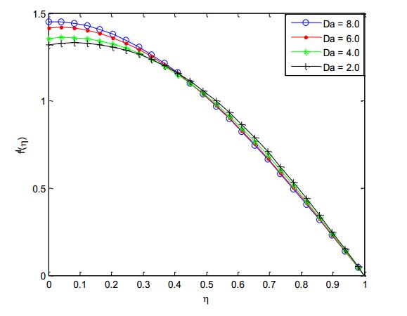
Effects of Darcy number on the flow pattern of the Casson nanofluid between the two parallel plates is portrayed in Figure 4. The figure displays an opposite trend to that of the squeezing number effects on the flow. It could be seen from the figure that as the Darcy number increases, the velocity increases in the range of \(0 \mathrm\le\eta\mathrm\le 0.5\) and then decreases in the range \(0.5 \mathrm< \eta\mathrm\le 1.\)
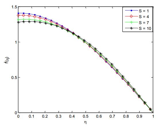
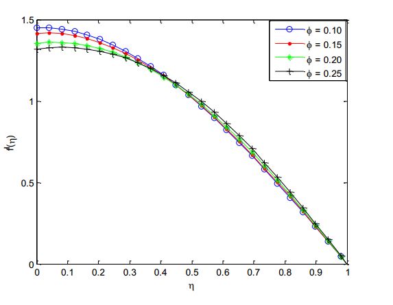
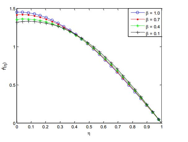
Figure 5 displays the effects of squeezing number on the flow behavior of the fluid. It is clear from the figure that as the squeezing number increases, the velocity decreases in the range of \(0 \mathrm\le\eta\mathrm\le 0.5\) and then increases in the range \(0.5 \mathrm< \eta\mathrm\le 1.\) Effect of nanoparticle fraction on the fluid velocity is depicted in Figure 6. The result shows that as the solid volume fraction of the fluid increases the velocity decreases in the range of \(0 \mathrm\le \eta\mathrm\le 0.5\) and then increases in the range 0.5 \(\mathrm{< }\) \(\eta\) \(\mathrm{\le}\) 1. This is because as the nanoparticle volume increases, more collision occurs between nanoparticle and particles with the boundary surface of the plates and consequently the resulting flow retardation which decreases the fluid velocity near the boundary layer. The flow behaviour of the Casson nanofluid to increasing Casson fluid parameter is shown in Figure 7. The figure depicts the effects of Casson fluid parameter on velocity profile of Casson nanofluid. It is obvious from the figure that Casson the parameter has influence on axial velocity. From the figure, it is clear that the magnitude of velocity of the fluid decreases in the range of 0 \(\mathrm{\le}\) \(\eta\) \(\mathrm{\le}\) 0.5 and then increases in the range 0.5 \(\mathrm{< }\) \(\eta\) \(\mathrm{\le}\) 1 as the Casson fluid parameter increases.
6. Conclusion
In this work, magnetohydrodynamic squeezing flow of nanofluid between two plates has been analyzed using differential transformation method. The results of the analytical solutions as developed in this study are agreement with the results of the numerical method using fourth-fifth order Runge-Kutta-Fehlberg method. Therefore, the obtained analytical solutions were used to investigate the squeezing phenomena of the nanofluid between the moving plates. Also, the effects of the pertinent flow parameters on the flow process were established. The results in this work can be used to further the study of squeezing flow in applications such as power transmission, polymer processing and hydraulic lifts.
Author Contributions
All authors contributed equally to the writing of this paper. All authors read and approved the
final manuscript.
Competing Interests
The author(s) do not have any competing interests in the manuscript.
References
Stefan, J. (1874). Versuche über die Scheinbare Adhäsion, Sitzungsberichte der Kaiserlichen Akademie der Wissenschaften, Mathematisch Naturwissenschaftliche Classe, vol. 69. Abteilung Wien.[Google Scholor]
Reynolds, O. (1886). IV. On the theory of lubrication and its application to Mr. Beauchamp tower’s experiments, including an experimental determination of the viscosity of olive oil. Philosophical Transactions of the Royal Society of London, (177), 157-234. [Google Scholor]
Archibald, F. R. (1965). Load capacity and time relations for squeeze films. Trans. Asme, 78, A231-A245. [Google Scholor]
Jackson, J. D. (1963). A study of squeezing flow. Applied Scientific Research, Section A, 11(1), 148-152. [Google Scholor]
Usha, R., & Sridharan, R. (1996). Arbitrary squeezing of a viscous fluid between elliptic plates. Fluid Dynamics Research, 18(1), 35-51. [Google Scholor]
Wolfe, W. A. (1965). Squeeze film pressures. Applied Scientific Research, Section A, 14(1), 77-90. [Google Scholor]
Kuzma, D. C. (1968). Fluid inertia effects in squeeze films. Applied Scientific Research, 18(1), 15-20. [Google Scholor]
Tichy, J. A., & Winer, W. O. (1970). Inertial considerations in parallel circular squeeze film bearings. Journal of Lubrication Technology, 92(4), 588-592. [Google Scholor]
Grimm, R. J. (1976). Squeezing flows of Newtonian liquid films an analysis including fluid inertia. Applied Scientific Research, 32(2), 149-166. [Google Scholor]
Birkoff, G. (1955). Hydrodynamics: a study in logic, fact and similitude. Dover. [Google Scholor]
Wang, C. Y. (1976). The squeezing of a fluid between two plates. Journal of Applied Mechanics, 43(4), 579-583. [Google Scholor]
Wang, C. Y., & Watson, L. T. (1979). Squeezing of a viscous fluid between elliptic plates. Applied Scientific Research, 35(2-3), 195-207.
[Google Scholor]
Hamdan, M. H., & Barron, R. M. (1992). Analysis of the squeezing flow of dusty fluids. Applied Scientific Research, 49(4), 345-354.
[Google Scholor]
Phan-Thien, N. (2000). Squeezing flow of a viscoelastic solid. Journal of Non-Newtonian Fluid Mechanics, 95(2-3), 343-362.[Google Scholor]
Khan, U., Ahmed, N., Khan, S. I. U., Bano, S., & Mohyud-Din, S. T. (2014). Unsteady squeezing flow of a Casson fluid between parallel plates. World Journal of Modelling and Simulation, 10(4), 308-319. [Google Scholor]
Rashidi, M. M., Shahmohamadi, H., & Dinarvand, S. (2008). Analytic approximate solutions for unsteady two-dimensional and axisymmetric squeezing flows between parallel plates. Mathematical Problems in Engineering, 2008, 1-13.[Google Scholor]
Duwairi, H. M., Tashtoush, B., & Damseh, R. A. (2004). On heat transfer effects of a viscous fluid squeezed and extruded between two parallel plates. Heat and mass transfer, 41(2), 112-117. [Google Scholor]
Qayyum, A., Awais, M., Alsaedi, A., & Hayat, T. (2012). Squeezing flow of non-Newtonian second grade fluids and micro polar models. Chinese Physics Letters, 29, 034701.
[Google Scholor]
Hamdan, M. H., & Barron, R. M. (1992). Analysis of the squeezing flow of dusty fluids. Applied Scientific Research, 49(4), 345-354. [Google Scholor]
Mahmood, M., Asghar, S., & Hossain, M. A. (2007). Squeezed flow and heat transfer over a porous surface for viscous fluid. Heat and mass Transfer, 44(2), 165-173. [Google Scholor]
Hatami, M., & Jing, D. (2016). Differential Transformation Method for Newtonian and non-Newtonian nanofluids flow analysis: Compared to numerical solution. Alexandria Engineering Journal, 55(2), 731-739. [Google Scholor]
Mohyud-Din, S. T., Zaidi, Z. A., Khan, U., & Ahmed, N. (2015). On heat and mass transfer analysis for the flow of a nanofluid between rotating parallel plates. Aerospace Science and Technology, 46, 514-522.[Google Scholor]
Mohyud-Din, S. T., & Khan, S. I. (2016). Nonlinear radiation effects on squeezing flow of a Casson fluid between parallel disks. Aerospace Science and Technology, 48, 186-192. [Google Scholor]
Qayyum, M., Khan, H., Rahim, M. T., & Ullah, I. (2015). Modeling and analysis of unsteady axisymmetric squeezing fluid flow through porous medium channel with slip boundary. PloS one, 10(3), e0117368. [Google Scholor]
Qayyum, M., & Khan, H. (2016). Behavioral study of unsteady squeezing flow through porous medium. Journal of Porous Media, 19(1), 83-94.[Google Scholor]
Mustafa, M., Hayat, T., & Obaidat, S. (2012). On heat and mass transfer in the unsteady squeezing flow between parallel plates. Meccanica, 47(7), 1581-1589. [Google Scholor]
Siddiqui, A. M., Irum, S., & Ansari, A. R. (2008). Unsteady squeezing flow of a viscous MHD fluid between parallel plates, a solution using the homotopy perturbation method. Mathematical Modelling and Analysis, 13(4), 565-576. [Google Scholor]
Domairry, G., & Aziz, A. (2009). Approximate analysis of MHD squeeze flow between two parallel disks with suction or injection by homotopy perturbation method. Mathematical Problems in Engineering, 2009, 603-616. [Google Scholor]
Acharya, N., Das, K., & Kundu, P. K. (2016). The squeezing flow of Cu-water and Cu-kerosene nanofluids between two parallel plates. Alexandria Engineering Journal, 55(2), 1177-1186.[Google Scholor]
Ahmed, N., Khan, U., Khan, S. I., Xiao-Jun, Y., Zaidi, Z. A., & Mohyud-Din, S. T. (2013). Magneto hydrodynamic (MHD) squeezing flow of a Casson fluid between parallel disks. International Journal of Physical Sciences, 8(36), 1788-1799. [Google Scholor]
Ahmed, N., Khan, U., Zaidi, Z. A., & Jan, S. U. (2014). A. Waheed, A., Mohyud-Din, ST, MHD Flow of a Dusty Incompressible Fluid between Dilating and Squeezing Porous Walls. Journal of Porous Media, Begal House, 17(10), 861-867. [Google Scholor]
Khan, U., Ahmed, N., Khan, S. I., Zaidi, Z. A., Xiao-Jun, Y., & Mohyud-Din, S. T. (2014). On unsteady two-dimensional and axisymmetric squeezing flow between parallel plates. Alexandria Engineering Journal, 53(2), 463-468.[Google Scholor]
Khan, U., Ahmed, N., Zaidi, Z. A., Asadullah, M., & Mohyud-Din, S. T. (2014). MHD squeezing flow between two infinite plates. Ain Shams Engineering Journal, 5(1), 187-192.[Google Scholor]
Hayat, T., Yousaf, A., Mustafa, M., & Obaidat, S. (2012). MHD squeezing flow of second-grade fluid between two parallel disks. International Journal for Numerical Methods in Fluids, 69(2), 399-410. [Google Scholor]
KKhan, H., Qayyum, M., Khan, O., & Ali, M. (2016). Unsteady squeezing flow of Casson fluid with magnetohydrodynamic effect and passing through porous medium. Mathematical Problems in Engineering, 2016, 4293721. [Google Scholor]
Ullah, I., Rahim, M. T., Khan, H., & Qayyum, M. (2016). Analytical analysis of squeezing flow in porous medium with MHD effect. University of Bucharest Scientific Bulletin Series A. Applied Mathematics and Physics, 78(2), 1223-7027. [Google Scholor]
Casson, N. (1959). Rheology of Dispersed System. 84, Pergamon Press, Oxford, UK.
Casson, N. (1959). A flow equation for the pigment oil suspension of the printing ink type. In: Rheology of
Disperse Systems, pp. 84-102. Pergamon, New York.[Google Scholor]
Dash, R. K., Mehta, K. N., & Jayaraman, G. (1996). Casson fluid flow in a pipe filled with a homogeneous porous medium. International Journal of Engineering Science, 34(10), 1145-1156. [Google Scholor]
Andersson, H.I., Dandapat, B.S. (1992). Flow of a power-law fluid over a stretching sheet. Applied Analysis of
Continuous Media, 1(339). [Google Scholor]
Sajid, M., Ahmad, I., Hayat, T., & Ayub, M. (2009). Unsteady flow and heat transfer of a second grade fluid over a stretching sheet. Communications in Nonlinear Science and Numerical Simulation, 14(1), 96-108.[Google Scholor]
Vlachopoulos, C., O’Rourke, M., & Nichols, W. W. (2011). McDonald’s blood flow in arteries: theoretical, experimental and clinical principles. CRC press.[Google Scholor]
Khan, U., Ahmed, N., Khan, S. I. U., Bano, S., & Mohyud-Din, S. T. (2014). Unsteady squeezing flow of a Casson fluid between parallel plates. World Journal of Modelling and Simulation, 10(4), 308-319. [Google Scholor]
Mustafa, M., Hayat, T., Pop, I., & Aziz, A. (2011). Unsteady boundary layer flow of a Casson fluid due to an impulsively started moving flat plate. Heat Transfer-Asian Research, 40(6), 563-576.[Google Scholor]
Hayat, T., Shehzad, S. A., Alsaedi, A., & Alhothuali, M. S. (2012). Mixed convection stagnation point flow of Casson fluid with convective boundary conditions. Chinese Physics Letters, 29(11), 114704. [Google Scholor]
Mukhopadhyay, S. (2013). Effects of thermal radiation on Casson fluid flow and heat transfer over an unsteady stretching surface subjected to suction/blowing. Chinese Physics B, 22(11), 114702.[Google Scholor]
Mukhopadhyay, S., De, P. R., Bhattacharyya, K., & Layek, G. C. (2013). Casson fluid flow over an unsteady stretching surface. Ain Shams Engineering Journal, 4(4), 933-938.[Google Scholor]
Mabood, F., Shateyi, S., & Khan, W. A. (2015). Effects of thermal radiation on Casson flow heat and mass transfer around a circular cylinder in porous medium. The European Physical Journal Plus, 130(9), 188. [Google Scholor]
Bhattacharyya, K. (2013). Boundary layer stagnation-point flow of casson fluid and heat transfer towards a shrinking/stretching sheet. Frontiers in Heat and Mass Transfer (FHMT), 4(2), 023003. [Google Scholor]
Pramanik, S. (2014). Casson fluid flow and heat transfer past an exponentially porous stretching surface in presence of thermal radiation. Ain Shams Engineering Journal, 5(1), 205-212. [Google Scholor]
Shateyi, S. (2013). A new numerical approach to MHD flow of a Maxwell fluid past a vertical stretching sheet in the presence of thermophoresis and chemical reaction. Boundary Value Problems, 2013(1), 196.
[Google Scholor]
Makanda, G., Shaw, S., & Sibanda, P. (2015). Effects of radiation on MHD free convection of a Casson fluid from a horizontal circular cylinder with partial slip in non-Darcy porous medium with viscous dissipation. Boundary Value Problems, 2015(1), 75.[Google Scholor]
Khalid, A., Khan, I., & Shafie, S. (2015). Exact solutions for unsteady free convection flow of Casson fluid over an oscillating vertical plate with constant wall temperature. Abstract and Applied Analysis 2015, 946350.[Google Scholor]
Eldabe, N. T. M., Saddeck, G., & El-Sayed, A. F. (2001). Heat transfer of MHD non-Newtonian Casson fluid flow between two rotating cylinders. Mechanics and Mechanical Engineering, 5(2), 237-251.[Google Scholor]
Nadeem, S., Haq, R. U., Akbar, N. S., & Khan, Z. H. (2013). MHD three-dimensional Casson fluid flow past a porous linearly stretching sheet. Alexandria Engineering Journal, 52(4), 577-582. [Google Scholor]
Zhou, J.K. (1986). Differential Transformation and Its Applications for Electrical Circuits. Huazhong
University Press, Wuhan, (in Chinese). [Google Scholor]