Open Journal of Mathematical Sciences

Vol. 4 (2020), Issue 1, pp. 386 – 396
ISSN: 2523-0212 (Online) 2616-4906 (Print)
DOI: 10.30538/oms2020.0128

Bayesian latent autoregressive stochastic volatility: an application of naira to eleven exchangeable currencies rates

R. O. Olanrewaju$^1$, J. F. Ojo, L. O. Adekola
Department of Statistics, University of Ibadan, 200284, Nigeria.; (R.O.O & J.F.O)
Department of Physical Sciences, the Bells University of Technology, Ota, Nigeria.; (L.O.A)
$^{1}$Corresponding Author: rasakiolawale@gmail.com

Copyright © 2020 R. O. Olanrewaju, J. F. Ojo, L. O. Adekola. This is an open access article distributed under the Creative Commons Attribution License, which permits unrestricted use, distribution, and reproduction in any medium, provided the original work is properly cited.

Received: July 28, 2020 – Accepted: November 9, 2020 – Published: November 28, 2020

Abstract

This paper provides a procedure for estimating Stochastic Volatility (SV) in financial time series via latent autoregressive in a Bayesian setting. A Gaussian distributional combined prior and posterior of all hyper-parameters (autoregressive coefficients) were specified such that the Markov Chain Monte Carlo (MCMC) iterative procedure via the Gibbs and Metropolis-Hasting sampling method was used in estimating the resulting exponentiated forms (quadratic forms) from the posterior kernel density. A case study of Naira to eleven (11) exchangeable currencies$^,$ rates by Central Bank of Nigeria (CBN) was subjected to the estimated solutions of the autoregressive stochastic volatility. The posterior volatility estimates at 5%, 50%, and 95% quantiles of ${e^{\frac{\mu }{2}}}$ = (0.130041, 0.1502 and 0.1795) respectively unveiled that the Naira-US Dollar exchange rates has the highest rates bartered by fluctuations.

Keywords:

Bayesian, gaussian, latent autoregressive, stochastic volatility (sv), markov chain monte carlo (mcmc).

1. Introduction

Volatility in financial time series returns came to existence some years back when [1] used it to estimate optimal expected time-varying volatilities (Variance trade-off) in portfolio construction. In time series, this volatility has been referred to as Stochastic Volatility or Stochastic Variance (SV) by [2]. Its application of interest ranges majorly from financial analyzes (econometrics), signal processing, telecommunications, mathematical sciences etc., in determining level of time-varying fluctuations [3]. SV models are as either Volatility Deterministic Models (VDMs) or Volatility Probabilistic Models (VDMs) [4,5].

The latter is strictly for Autoregressive (AR) state-space like models (latent Markov model) where the natural logarithms of the squared volatilities of return assets are of interest [6]. The formal type models are models with trait of time-varying volatility of asset returns via Autoregressive Conditional Heteroscedasticity (ARCH) type models, that is, ARCH and Generalized Autoregressive Conditional Heteroscedasticity (GARCH) model proposed by [7,8] for classifying volatility (variance) as a random process. The deterministic SV ARCH type models are usually affected by leverage effect for not taken into consideration asymmetrical traits of volatility of financial assets that do not typically and fully reflect in the risk in [9]. In contrast to either positive or negative estimate of volatility estimates, estimates in ARCH models are usually constrained to positive values (see [10,11]). Having said this, the error term in SV models also followed two types of processes - Observation and Latent Volatility Processes. Latent volatility process goes in line with the deterministic variance models while the observation process is in support of the probabilistic volatility models.

Among the numerous methods of overcoming the challenge of parameter estimation of SV with both error terms (probabilistic volatility models) and deterministic variance models are via Maximum Likelihood (ML), Method of Moments (MM), Simulated Method of Moments (SMM) and Simulated Maximum Likelihood (SML), Quasi-Maximum Likelihood (QML) and Generalized Method of Moments (GMM) [12,13]. Notable setback to these methods of estimating volatilities of financial asset returns has been non-adaptable to approximation error and zigzag efficiency gain of these likelihood-based approaches [14]. To circumnavigate these problems, article [15] started the conformation and modification to the latent SV products via Exponentially Weighted Moving Average (EWMA) estimated scaled absolute returns via calibrated weights. In a similar vein, article [16] analyzed the class of continuous-time jump diffusion of stochastic volatility via Levy $\alpha $-stable (compound Poisson) MCMC. Furthermore, article [17] modeled the SV model assuming student-t-distributed errors and revealed efficiency gains by Markov Chain Monte Carlo (MCMC) methods in comparison with GMM. In this regard, this paper employed the Bayesian MCMC of a latent (state-space) autoregressive SV model via simplified multivariate posterior distribution. A combined Gaussian prior was specified for the variance (volatility) including the hyper-parameters for a posterior form that was streamlined down to Gibbs and Metropolis-Hasting sampling method of iterative procedure. However, the estimated solutions were subjected to exchange rates of Naira to ten (10) most exchangeable currencies from 2012 to May 2018 as well as a Special Drawing Right (SDR) reserved exchange rates for world transactions by International Monetary Fund (IMF).

2. Specification of the latent autoregressive stochastic volatility

Let ${x_t} = \,{({x_1},{x_2}, \ldots \ldots ,{x_n})^T} \in \Re$ be a vector of stochastic process of logarithm returns of latent volatility model, then

\begin{equation}\label{e1} {x_t} = \,{\sigma _t}{\varepsilon _t}\hspace{5em} for\,\,\,\,t \in \, N\,, \end{equation}

(1)

such that $ \,\,{\varepsilon _t}\, \sim \,N(0,\,\sigma _\varepsilon ^2)$, then the volatility series of ${y_t}$ is nothing but the time-varying conditional variance of the squared stochastic process given the latent variable ${h_t}$, $\sigma _t^2 = E(y_t^2/\,{h_t})$ such that the standard deviation is

\begin{equation}\label{e2} {\sigma _t} = \,{e^{\left( {\frac{{h{\,_t}}}{2}} \right)}}\,. \end{equation}

(2)

For ${h_t} = \,{\left\{ {{x_{t - 1}},{x_{ - 2}}, \ldots \ldots } \right\}^`}$ and latent like Autoregressive model

\begin{equation}\label{e3} {h_t} = \,\mu + \,{\phi _1}({h_{t - 1}} - \mu ) + \,{\omega _t}\hspace{5em} t = 2,\,3, \ldots\,, \end{equation}

(3)

where ${h_t}$ follows the normal distribution of the white noise ${w_t} \sim N(0,\,{\sigma ^2})$. So parameterizing \[ {y_t}/\,{h_t}\, \sim \,N\left( {0,\,\sigma _\varepsilon ^2{e^{({h_{\,t}})}}} \right)\,.\]

\begin{equation}\label{e4} {h_{\,\,t}}/\,{h_{t - 1}},\,\mu ,\,\phi ,\,{\sigma _\omega } \sim N\left( {{h_t} = \,\mu + \,\phi ({h_{t - 1}} - \mu ),\,\sigma _\omega ^2} \right) \end{equation}

(4)

\[ {h_0}/\,\mu ,\,\phi ,\,\sigma _\varepsilon ^2 \sim N\left( {\mu ,\,\frac{{\sigma _\omega ^2}}{{1 - \phi _1^2}}} \right)\,.\] For mean and variance of Autoregressive model as defined by [7,9] as $E({h_t}) = \mu $ and ${var} ({h_t}) = \frac{{\sigma _\varepsilon ^2}}{{1 + {\phi _1}\rho }}$ for autocorrelation coefficient ''$\rho $'' of order one and probability function $g( . )\,.$

In general, Equation (3) can be re-written as

\begin{equation}\label{e5} {h_t} = \,\mu + \,\sum\limits_{i = 1}^p {\mu + \,{\phi _i}({h_{t - 1}} - \mu )} + \,{\omega _t}\,, \end{equation}

(5)

for order ''$\rho $'' and stationary process of $0 < \,{\phi _i} < 1$ where $\phi = \,{\phi _i} = {\left\{ {{\phi _1},{\phi _2}, \ldots, {\phi _p}} \right\}^,}\,.$

3. Prior specification

From Equation (5), $\phi $ lies between $\left( { - 1,\,1} \right)$, because of the vector's range, it suggested an informative prior distribution of Beta distribution, i.e., $\phi \sim { B}(a,b)$

\begin{equation}\label{e6} p(\phi ) = \,\frac{1}{{2B(a,b)}}\,{\left( {\frac{{1 + \phi }}{2}} \right)^{a - 1}}{\left( {\frac{{1 - \phi }}{2}} \right)^{b - 1}}\,, \end{equation}

(6)

with $E(\phi ) = \frac{a}{{a + b}}$, $v\,(\phi ) = \,\frac{{4ab}}{{{{(a + b)}^2}(a + b + 1)}}$, $\sigma _\omega ^2$ and ${\omega _t}$ follows an Inverted Gamma (IG) distribution

\begin{equation}\label{e7} p(\sigma _\omega ^2) = \frac{{{{\left( {\sigma _\omega ^2} \right)}^{ - ({a_2} + 1)}}{e^{ - \frac{1}{{{b_2}\,\sigma _\omega ^2}}}}}}{{\Gamma ({a_2})\,{{\left( {{b_2}} \right)}^{{a_2}}}}};\,\,\,\,\,\,\,\,\,\,\,\,\sigma _\omega ^2 > 0\,, \end{equation}

(7)

with $E(\sigma _\omega ^2) = \frac{{{b_2}}}{{{a_2} - 1}}$, $v(\sigma _\omega ^2) = \frac{{b_2^2}}{{\left( {{{({a_2} - 1)}^2}({a_2} - 2)} \right)}}$ such that $\sigma _\omega ^2 \sim IG({a_2},\,{b_2})$ $\sigma _\varepsilon ^2 \sim IG({a_3},\,{b_3})$ at ${h_t} = 0,$ $t - i = 0,\, - 1,\, - 2,\, - 3,\, \ldots \ldots , - \rho + 1\,.$

4. Parameter estimation

Since the distribution of ${h_t}$ follows the same distribution with $\mu \sim N(0,\,{\varepsilon ^2})$, then conditional distribution of ${h_t}$ is

\begin{equation}\label{e8} g({h_t}/{h_{t - 1}}) = \,\frac{1}{{{{\left( {2\pi \sigma _\omega ^2} \right)}^{\frac{1}{2}}}}}e\left\{ { - \frac{1}{{2\sigma _\omega ^2}}{{\left( {{h_t} - \mu - \sum\limits_{i = 1}^p {{\phi _i}({h_{t - i}} - \mu )} } \right)}^2}} \right\}\,. \end{equation}

(8)

So, based on the intend hyper-parameters to be estimated, independent prior distributions can be carved out based on $\phi = {({\phi _1},{\phi _2}, \ldots,{\phi _p})^T}\ $, ${h_t} = \,{({h_1},{h_2}, \ldots,{h_{n - p}})^T}$,$\sigma _\omega ^2$, $\,\sigma _\varepsilon ^{2}$, and $\mu $. However, a combined prior distribution will be employed by via $\xi = \left\{ {\phi ,h,\sigma _\omega ^2,\sigma _\varepsilon ^{2},\mu } \right\}$

\begin{equation}\label{e9} g(\xi /x) = \prod\limits_{i = 1}^n {\frac{1}{{{{\left( {2\pi \sigma _\varepsilon ^2{e^{({h_t})}}} \right)}^{\frac{1}{2}}}}}{e^{ - \left\{ {\frac{{x_t^2}}{{2\pi \sigma _\varepsilon ^2{e^{({h_t})}}}}} \right\}}}} \frac{1}{{\sqrt {2\pi \sigma _\varepsilon ^2} }}{e^{ - \frac{1}{{2\sigma _\omega ^2}}{{\left[ {{h_t} - \mu - \sum\limits_{i = 1}^p {{\phi _i}({h_{t - i}} - \mu )} } \right]}^2}}} \end{equation}

(9)

$\times \,\,\,\text{combined}\,g(\xi )$. The combined prior is the combine kernel form of all the hyper-parameters given as

\begin{equation}\label{e10} g(\xi )\infty \left( {\prod\limits_{i = 1}^n {\phi _i^{{a_{i - 1}}}} {{(1 - {\phi _i})}^{{b_i}}}} \right){\left( {\sigma _\omega ^2} \right)^{ - \frac{{{a_2} + 1}}{2}}}e\left\{ { - \frac{{{b_2}}}{{\sigma _\omega ^2}}} \right\}\,{\left( {\sigma _\varepsilon ^2} \right)^{ - \frac{{{a_3} + 1}}{2}}}e\left\{ { - \frac{{{b_3}}}{{\sigma _\varepsilon ^2}}} \right\}e\left\{ { - \frac{{{\mu ^2}}}{{2{\varepsilon ^2}}}} \right\}\,. \end{equation}

(10)

The posterior,

\begin{eqnarray} \label{e11} &&\notag g(\xi /x) = \,\left( {\frac{1}{{\sqrt {2\pi \sigma _\varepsilon ^2} }}} \right){e^{ - \frac{1}{2}\left[ {{h_1} - \frac{1}{{2\sigma _\varepsilon ^2}}\,x_1^2{e^{ - {h_{\,1}}}}} \right]}}\, \times\left( {\frac{1}{{\sqrt {2\pi \sigma \,_\varepsilon ^2} }}} \right){e^{ - \frac{1}{2}\left[ {{h_{\,2}} - \frac{1}{{2\sigma _\varepsilon ^2}}\,x_2^2{e^{ - {h_{\,2}}}}} \right]}}\times \cdots\&&\notag \times \left( {\frac{1}{{\sqrt {2\pi \sigma _\varepsilon ^2} }}} \right){e^{ - \frac{1}{2}\left[ {{h_{\,n}} - \,\frac{1}{{2\sigma _\varepsilon ^2}}\,x_n^2\,{e^{ - {h_{\,n}}}}} \right]}} \times \left( {\frac{1}{{\sqrt {2\pi \sigma _\omega ^2} }}} \right){e^{ - \frac{1}{{2\sigma _\omega ^2}}{{\left( {{h_{\,1}} - \mu - \sum\limits_{i = 1}^p {{\phi _i}({h_{\,1 - i}} - \mu )} } \right)}^2}}}\\ &&\times\left( {\frac{1}{{\sqrt {2\pi \sigma _\omega ^2} }}} \right){e^{ - \frac{1}{{2\sigma _\omega ^2}}{{\left( {{h_{\,2}} - \mu - \sum\limits_{i = 1}^p {{\phi _i}({h_{\,2 - i}} - \mu )} } \right)}^2}}} \times \cdots\times \left( {\frac{1}{{\sqrt {2\pi \sigma _\omega ^2} }}} \right){e^{ - \frac{1}{{2\sigma _\omega ^2}}{{\left( {{h_{\,n}} - \mu - \sum\limits_{i = 1}^p {{\phi _i}({h_{\,n - i}} - \mu )} } \right)}^2}}} \notag\\&&\times \,\,\,g(\xi )\,, \end{eqnarray}

(11)

\begin{eqnarray} \label{e12}&&\notag g(\xi /x) = {\left( {2\pi } \right)^{ - \frac{1}{2}}}\,{\left( {\sigma _\varepsilon ^2} \right)^{ - \frac{1}{2}}}{e^{ - \frac{1}{2}\left[ {{h_1} - \frac{1}{{2\sigma _\varepsilon ^2}}\,x_1^2{e^{ - {h_1}}}} \right]}}\times {\left( {2\pi } \right)^{ - \frac{1}{2}}}\,{\left( {\sigma _\varepsilon ^2} \right)^{ - \frac{1}{2}}}{e^{ - \frac{1}{2}\left[ {{h_2} - \frac{1}{{2\sigma _\varepsilon ^2}}\,x_2^2{e^{ - {h_2}}}} \right]}}\times \cdots\\ &&\notag \times {\left( {2\pi } \right)^{ - \frac{1}{2}}}\,{\left( {\sigma _\varepsilon ^2} \right)^{ - \frac{1}{2}}}{e^{ - \frac{1}{2}\left[ {{h_n} - \frac{1}{{2\sigma _\varepsilon ^2}}\,x_n^2{e^{ - {h_n}}}} \right]}} \times \,{\left( {2\pi } \right)^{ - \frac{1}{2}}}\,{\left( {\sigma _\omega ^2} \right)^{ - \frac{1}{2}}}{e^{ - \frac{1}{{2\sigma _\omega ^2}}{{\left( {{h_{\,1}} - \mu - \sum\limits_{i = 1}^p {{\phi _i}({h_{\,1 - i}} - \mu )} } \right)}^2}}}\\ && \times {\left( {2\pi } \right)^{ - \frac{1}{2}}}\,{\left( {\sigma _\omega ^2} \right)^{ - \frac{1}{2}}}{e^{ - \frac{1}{{2\sigma _\omega ^2}}{{\left( {{h_{\,2}} - \mu - \sum\limits_{i = 1}^p {{\phi _i}({h_{\,2 - i}} - \mu )} } \right)}^2}}} \times \cdots \times{\left( {2\pi } \right)^{ - \frac{1}{2}}}\,{\left( {\sigma _\omega ^2} \right)^{ - \frac{1}{2}}}{e^{ - \frac{1}{{2\sigma _\omega ^2}}{{\left( {{h_{\,n}} - \mu - \sum\limits_{i = 1}^p {{\phi _i}({h_{\,n - i}} - \mu )} } \right)}^2}}}\notag\\&& \times g(\xi )\,. \end{eqnarray}

(12)

Factoring out the constants,

\begin{eqnarray*} &&\notag g(\xi /x) = {\left( {2\pi } \right)^{ - \frac{n}{2}}}\,{\left( {\sigma _\varepsilon ^2} \right)^{ - \frac{n}{2}}}\times{e^{ - \frac{1}{2}\left[ {{h_1} - \frac{1}{{2\sigma _\varepsilon ^2}}\,x_1^2{e^{ - {h_1}}}} \right]}}{e^{ - \frac{1}{2}\left[ {{h_2} - \frac{1}{{2\sigma _\varepsilon ^2}}\,x_2^2{e^{ - {h_2}}}} \right]}} \times\cdots \\ &&\notag \times{e^{ - \frac{1}{2}\left[ {{h_n} - \frac{1}{{2\sigma _\varepsilon ^2}}\,x_n^2{e^{ - {h_n}}}} \right]}} \times \,{\left( {2\pi } \right)^{ - \frac{n}{2}}}\,{\left( {\sigma _\omega ^2} \right)^{ - \frac{n}{2}}}{e^{ - \frac{1}{{2\sigma _\omega ^2}}{{\left( {{h_{\,1}} - \mu - \sum\limits_{i = 1}^p {{\phi _i}({h_{\,1 - i}} - \mu )} } \right)}^2}}}{e^{ - \frac{1}{{2\sigma _\omega ^2}}{{\left( {{h_{\,2}} - \mu - \sum\limits_{i = 1}^p {{\phi _i}({h_{\,2 - i}} - \mu )} } \right)}^2}}} \end{eqnarray*} \begin{eqnarray} \label{e13} && \times\cdots \cdots \times{e^{ - \frac{1}{{2\sigma _\omega ^2}}{{\left( {{h_{\,n}} - \mu - \sum\limits_{i = 1}^p {{\phi _i}({h_{\,n - i}} - \mu )} } \right)}^2}}} \times g(\xi )\,. \end{eqnarray}

(13)

Regrouping for kernel density in Equation (12) gives;

\begin{equation}\label{e14} g(\xi /x) = C\,{\left( {\sigma _\varepsilon ^2} \right)^{ - \frac{n}{2}}}{e^{ - \frac{1}{2}\left[ {\sum\limits_{t = 1}^n {{h_t}} - \frac{1}{{2\sigma _\varepsilon ^2}}\sum\limits_{t = 1}^n {x_t^2} \,{e^{ - {h_t}}}} \right]}} \times \,{\left( {\sigma _\omega ^2} \right)^{ - \frac{n}{2}}} - \frac{1}{{2\sigma _\omega ^2}}{e^{\left[ {\sum\limits_{t = 1}^n {{{\left( {{h_{\,t}} - \mu - \sum\limits_{i = 1}^p {{\phi _i}({h_{\,t - i}} - \mu )} } \right)}^2}} } \right]}} \times \,g(\xi )\,, \end{equation}

(14)

where $C$ is overall constant after multiplication of resulting constants. In term of the proportionality, the posterior $g(\xi /y)$ becomes;

\begin{equation}\label{e15} g(\xi /x)\infty {\left( {\sigma _\varepsilon ^2} \right)^{ - \frac{n}{2}}}{e^{ - \frac{1}{2}\left[ {\sum\limits_{t = 1}^n {{h_t}} - \frac{1}{{2\sigma _\varepsilon ^2}}\sum\limits_{t = 1}^n {x_t^2} \,{e^{ - {h_t}}}} \right]}} \times \,{\left( {\sigma _\omega ^2} \right)^{ - \frac{n}{2}}} - \frac{1}{{2\sigma _\omega ^2}}{e^{\left[ {\sum\limits_{t = 1}^n {{{\left( {{h_{\,t}} - \mu - \sum\limits_{i = 1}^p {{\phi _i}({h_{\,t - i}} - \mu )} } \right)}^2}} } \right]}} \times \,g(\xi )\,. \end{equation}

(15)

The two exponent terms (quadratic forms) inside ${\left[ {\,\,\,\,\,} \right]^,}s$ above can expand and compress to a multivariate matrix of a Multivariate Normal densities, since the posterior distribution fall back to give the form of the prior (conjugate prior), i.e.,

\begin{equation}\label{e16} g(\xi /x)\infty {\left( {\sigma _\varepsilon ^2} \right)^{ - \frac{n}{2}}}{e^{ - \frac{1}{2}\left[ {{I^{'\,}}H - \frac{1}{{2\sigma _\varepsilon ^2}}{X^!}\,\Sigma } \right]}} \times \,{\left( {\sigma _\omega ^2} \right)^{ - \frac{n}{2}}} - \frac{1}{{2\sigma _\omega ^2}}{e^{\left[ {{{\left( {H - \mu - {X^!}\phi } \right)}^!}\,\left( {H - \mu - {X^!}\phi } \right)} \right]}} \times \,g(\xi )\,, \end{equation}

(16)

where $I$ Is the identity matrix of unity of $n\,by\,1$. $\Sigma = \,\left( {{e^{ - {h_{\,1}}}}, \cdots \cdots {e^{ - {h_{\,n}}}}} \right)$, $H = {h_t}$ and $\phi $ are $n\,by\,1$ matrix as defined above, $\mu$ is a $n\,by\,1 $ vector matrix; $X$ is a $n\,by\,p$ square matrix of \[ \begin{array}{*{20}{c}} {{h_0}}&{{h_{ - 1}}}& \cdots &{{h_{ - p + 1}}} \\ {{h_1}}&{{h_0}}& \cdots &{{h_{ - p + 2}}} \\ \vdots & \vdots & \vdots & \vdots \\ {{h_{n - 1}}}&{{h_{n - 2}}}& \cdots &{{h_{n - p}}} \end{array}\,.\]

4.1. Markov chain monte carlo (MCMC) algorithms

Employing the MCMC iterative procedure proposed by [5] to solve Equation (16) via the Gibbs and Metropolis - Hasting sampling method;

1. Initializing ${h^{(0)}},\,\sigma _\varepsilon ^{2(0)},\,\sigma _\omega ^{2(0)},\,{\phi ^{(0)}}$ $i = 1$ by setting $i = 1$
2. Sample from $h_t^{(i)}$ from $g\left( {{h_t}/{h_{t - 1}},x,\,{\phi ^{(i - 1)}},\,{\mu ^{(i - 1)}},\,\sigma _\varepsilon ^{2(i - 1)},\sigma _\omega ^{2(i - 1)}} \right)$
3. Sample from ${\phi ^{(i)}}$ from $g\left( {{\phi ^{(i)}}/{h_t},x,\,{\mu ^{(i - 1)}},\,\sigma _\varepsilon ^{2(i - 1)},\sigma _\omega ^{2(i - 1)}} \right)$
4. Sample $\sigma _\omega ^{2(i)}$ from $g\left( {\sigma _\omega ^{2(i)}/{h_t},x,\,{\phi ^{(i - 1)}},\,{\mu ^{(i - 1)}},\,\sigma _\varepsilon ^{2(i - 1)}} \right)$
5. Sample from $\sigma _\varepsilon ^{2(i)}$ from $g\left( {\sigma _\varepsilon ^{2(i)}/{h_t},x,\,{\phi ^{(i - 1)}},\,{\mu ^{(i - 1)}},\,\sigma _\omega ^{2(i - 1)}} \right)$
6. Sample ${\mu ^{(i)}}$ from $g\left( {{\mu ^{(i)}}/{h_t},x,\,{\phi ^{(i - 1)}},\,\sigma _\omega ^{2(i - 1)},\sigma _\varepsilon ^{2(i - 1)}} \right)$
7. If $i < \,I$ , set $i = i + 1$ go to step two by repeating procedure /step 2 - 7, until convergence is reached, where $I$ is the number of iterations.

5. Result and discussions

The financial returns of Naira to eleven (10) currencies$^,$ exchange rates as well as a Special Drawing Right (SDR) reserved currency as stated by International Monetary Fund (IMF) from 2012 to May 31, 2018 was pinpointed as a case study. The exchangeable currencies weighted in amount measured per unit in valuation Nigeria$^,$ s naira by the Central Bank of Nigeria (CBN). The United States$^,$ currency, US Dollar ; the United Kingdom$^,$s currency, Pounds Sterling ; the European States$^,$ currency, Euro; the Switzerland$^,$s currency, Swiss Franc (SwF); the Japanese$^,$s currency, Yen ;the Communaute Financiere d$^,$Afrique (Financial Community of Africa) CFA franc currency uses by eight Francophone West African countries (Benin, Burkina Faso, Guinea - Bissau, Ivory Coast, Mali, Niger, Senegal and Togo); the Saudi Arabia$^,$ currency , Riyal (SAR); the Denmark$^,$s currency, Danish Krone (DKr); the Chinese$^,$s currency, Yuan / Renminbi (CNY, ) and the West African Union of Account (WAUA) legal tender cheque in the sub-region of ECOWAS member-countries. In addition is the Special Monetary Rights (SDR), a monetary reserve currency created by International Monetary Fund (IMF) to re-evaluate US Dollar, Euro, Chinese Yuan, Japanese Yen and Pound Sterling. SDR is a freely usable foreign currency in international transactions and foreign exchange markets. This reserve currency by IMF able staunch countries like Nigeria to borrow fund with a calculated exchange rate(s) and interest rate(s) based on economic indexes. The exchange rates of Naira to the mentioned currencies comprise of 2314 sample points of their exchange rates recorded by CBN.

Table 1. Descriptive statistics of the Naira - the currencies${^,}$ exchange rates.

Rates	Mean	SD	Median	Trimmed	MAD	Min.	Max.	Skew.	Kurt.	S.E
US$	215.98	65.65	196.50	212.27	61.17	154.25	324.50	0.51	-1.55	1.73
P.S	310.48	67.05	286.12	306.14	56.23	24.97	437.03	0.46	-1.19	1.76
EURO	256.59	66.82	215.48	249.97	19.17	187.37	410.59	0.72	-1.31	1.76
SwF	224.71	63.50	198.86	220.69	47.62	2.74	338.34	0.53	-1.42	1.67
Yen	2.02	0.57	1.67	1.98	0.27	1.34	3.23	0.58	-1.45	0.01
CFA	0.38	0.11	0.32	0.37	0.03	0.16	1.74	1.96	15.54	0.00
WAUA	308.21	85.84	272.26	302.18	54.73	24.85	455.36	0.53	-1.29	2.26
SAR	33.63	9.21	30.32	32.94	7.89	24.33	81.42	0.59	-1.05	0.24
CNY	57.43	17.61	52.38	56.50	16.29	22.87	86.50	0.50	-1.53	0.46
DKr	35.74	20.06	28.88	33.65	2.55	22.31	418.01	10.63	151.11	0.53
SDR	308.62	87.05	272.93	303.23	54.16	25.35	456.12	0.44	-1.10	2.29

Keys: MAD=Mean Absolute Deviation; Skew-Skeweness; Kurt=Kurtosis.

It is obvious from Table 1 that Pound Sterling (P.S) maintained the highest currency that shrinks the valuation of its exchange to naira followed by the Euro, Swiss Franc and US-Dollar ($) such that the CFA franc currency seemed to be the lowest valuation in exchange for Naira. The MAD indicated a highest susceptible measure of the variability in US-Dollar with a residuals${^,}$ deviation of 61.17% from the median of 196.50 over this period. Also, United Kingdom${^,}$s Pound Sterling, WAUA and SDR prone above average to the residual deviation of 56.23 %, 54.73% and 54.16 % from their respective medians of 286.12, 272.26 and 272.93. CFA and DKr exchange rates might like be the rates to be affected by tails of data point with their skewnesses (15.54 and 151.11) strictly greater than 3.

Figure 1. The Time Plots of Naira–the Currencies${^,}$ Exchange rates

From Figure 1, the exchange rates of US-Dollar, Pounds Sterling and Swiss Franc had a drastic fall to favor naira in exchange for their valuation around the second quarter of 2013. In contrast, the Euro maintained a sporadic uprising in the same second quarter of the 2013 for its exchange to be less valued in exchange for naira. The naira gained a significant profitable valuation in trading for US-Dollar, Pounds Sterling, Euro, Swiss Franc, CFA, Yen, SDR, Danish Krone and WAUA towards the end of first quarter in 2016 before skyrocketing back to their stringent rates from second stanza of 2016 to May 2018. It is to be noted that Saudi Arabia$^,$ s riyal and Chinese$^,$s Yuan perpetuated a burgeoning and dwindling rates before maintaining a constant level of settlement in trading with Naira from 2012 to mid-2018.

Table 2. Summary of Prior distributions.

$\mu$	Normal (Mean = -10, SD = 1)
$\frac{{{\phi _{ + 1}}}}{2}$	$\beta$ (a= 20, b= 1.1)
${\sigma ^2}$	0.1 * Chis-squared (d.f = 1)

Table 3. Posterior draws of parameters Naira - the Currencies${^,}$ exchange rates.

	$\mu$	-3.8055	0.7357	-4.0774	-3.8056	-3.8056	1354
	${\phi _1}$	0.3477	1.2315	3.2373	3.3477	3.4580	304
Naira- US Dollar	$\sigma $	2.1705	0.7850	1.8761	2.1337	2.575	120
	${e^{\frac{\mu }{2}}}$	0.1520	0.0559	0.1300	0.1502	0.1795	1354
	${\sigma ^2}$	1.2875	0.9473	0.9564	1.2507	1.8026	120
	$\mu$	-10.6786	0.10768	-10.8510	-10.6803	-10.5012	2277
	${\phi _1}$	0.6728	0.0473	0.5896	0.6752	0.7455	254
Naira- Pounds Sterling	$\sigma $	1.1720	0.0774	1.0489	1.1694	1.3045	242
	${e^{\frac{\mu }{2}}}$	0.0048	0.0003	0.0044	0.0048	0.0052	2277
	${\sigma ^2}$	1.3796	0.1824	1.1002	1.3676	1.7017	242
	$\mu$	-10.7180	0.0857	-10.8558	-10.7189	-10.577	1598
	${\phi _1}$	0.5124	0.0609	0.4121	0.5132	0.613	257
Naira- Euro	$\sigma $	1.2525	0.0749	1.1314	1.2516	1.375	304
	${e^{\frac{\mu }{2}}}$	0.0047	0.0002	0.0044	0.0047	0.005	1598
	${\sigma ^2}$	1.5743	0.1883	1.2801	1.5665	1.892	304
	$\mu$	-10.6573	0.09181	-10.8061	-10.6569	-10.5083	1884
	${\phi _1}$	0.5564	0.05309	0.4636	0.5599	0.6372	257
Naira-Swiss Franc	$\sigma $	1.2636	0.07196	1.1521	1.2589	1.3904	307
	${e^{\frac{\mu }{2}}}$	0.0049	0.0002	0.0045	0.0049	0.0052	1884
	${\sigma ^2}$	1.6018	0.18340	1.3272	1.5850	1.9333	307
	$\mu$	-10.3817	0.12459	-10.579	-10.3846	-10.1729	1613
	${\phi _1}$	0.8223	0.0525	0.725	0.8289	0.8950	82
Naira-Yen	$\sigma $	0.7187	0.0975	0.570	0.7124	0.8911	79
	${e^{\frac{\mu }{2}}}$	0.0056	0.00035	0.005	0.0056	0.0062	1613
	${\sigma ^2}$	0.5261	0.1439	0.325	0.5075	0.7940	79
	$\mu$	-10.9782	0.09980	-11.1454	-10.9756	-10.8158	1597
	${\phi _1}$	0.3823	0.04584	0.3073	0.3819	0.4569	462
Naira-CFA	$\sigma $	1.9453	0.07270	1.8261	1.9460	2.0637	392
	${e^{\frac{\mu }{2}}}$	0.0041	0.0002	0.0038	0.0041	0.0045	1597
	${\sigma ^2}$	3.7896	0.2828	3.3348	3.7870	4.2590	392
	$\mu$	-12.2891	0.10128	-12.454	-12.2893	-12.1219	2104
	${\phi _1}$	0.4398	0.04598	0.366	0.4387	0.5169	442
Naira-WAUA	$\sigma $	1.8360	0.06742	1.722	1.8375	1.9460	453
	${e^{\frac{\mu }{2}}}$	0.0021	0.00011	0.002	0.0021	0.0023	2104
	${\sigma ^2}$	3.3755	0.24724	2.964	3.3763	3.7868	453
	$\mu$	-12.3040	0.13271	-12.5208	-12.3054	-12.0882	2506
	${\phi _1}$	0.6694	0.03482	0.6110	0.6698	0.7260	491
Naira-Riyal	$\sigma $	1.5447	0.06280	1.4418	1.5449	1.6476	421
	${e^{\frac{\mu }{2}}}$	0.0021	0.00014	0.0019	0.0021	0.0024	2506
	${\sigma ^2}$	2.3902	0.19412	2.0787	2.3867	2.7144	421

Table 4. Posterior draws of parameters Naira - the Currencies${^,}$ exchange rates.

	$\mu$	-4.3492	0.59792	-16.1935	-4.3492	-4.0774	19
	${\phi _1}$	2.7959	0.0403	0.7080	2.7959	3.0166	95
Naira-Yuan / Renminbil	$\sigma $	2.0000	0.0763	1.848	2.000	2.100	254
	${e^{\frac{\mu }{2}}}$	0.0750	0.0002	0.0003	0.0659	0.1026	19
	${\sigma ^2}$	3.900	0.3009	3.4163	3.900	4.400	254
	$\mu$	-10.5755	0.1218	-10.7745	-10.5761	-10.3772	2982
	${\phi _1}$	0.5739	0.0413	0.5039	0.5757	0.6401	364
Naira-Danish Kronal	$\sigma $	1.7602	0.07204	1.6425	1.7592	1.8821	373
	${e^{\frac{\mu }{2}}}$	0.0051	0.0003	0.0046	0.0051	0.0056	2982
	${\sigma ^2}$	3.1037	0.2543	2.6977	3.0947	3.5423	373
	$\mu$	-12.0793	0.1166	-12.2689	-12.0805	11.8846	2829
	${\phi _1}$	0.4969	0.0396	0.4308	0.4975	0.5616	545
Naira-Danish Kronal	$\sigma $	2.0285	0.0666	1.9212	2.0271	2.1402	503
	${e^{\frac{\mu }{2}}}$	0.0024	0.0001	0.0022	0.0024	0.0026	2829
	${\sigma ^2}$	4.1193	0.2706	3.6911	4.1092	4.5803	503

From Table 2, the prior mean and variance from Equation (6) are estimated to be 1.24 and 0.070 respectively, suggesting more than 70% positive values of the Bayesian latent stationary process of the ${\phi ^,}s$ at lag one. Also, since $'a'$ and $'b'$ are approximately not equal to one, it connotes that the chosen informative prior of hyper-parameters did not clout the posterior${^,}$s parameters of 10000 MCMC iterative convergence. From Tables 3 and 4, all the autoregressive coefficients ${\phi ^,}s$\, $i = 1,2,3, \cdots ,11$ are less than one to ascertain and confirmed the stationarity processes of the 11 exchange rates. The posterior VS volatile estimates at 5%, 50%, and 95% quantiles of Naira--US Dollar exchange rates with their respective = (0.130041, 0.1502 and 0.1795) respectively been the highest level of fluctuation among the currencies under study. Next in the second cadre of category bartered by the evanescent Naira exchange rates at 5%, 50%, and 95% quantiles were the Japanese${^,}$s Yen, the Denmark${^,}$s Danish kroner, the Switzerland${^,}$s Swiss Franc, the United Kingdom${^,}$s Pounds sterling, United States${^,}$Euro and CFA franc currency uses by eight Francophone West African countries (Benin, Burkina Faso, Guinea-Bissau, Ivory Coast, Mali, Niger, Senegal and Togo) with their stochastic volatilities recorded has ${e^{\frac{\mu }{2}}}$ = (0.005, 0.0056, 0.0062), (0.0046, 0.0051, 0.0056 ), (0.0045, 0.0049, 0.0052), (0.0044, 0.0048, 0.0052), (0.0044, 0.0047, 0.005) and (0.0038, 0.0041,0.0045) respectively. The Chinese Yuan SV rates over this stipulated period of study sporadically skyrocketed at 95% quantile with 0.10256, moderately normal at 50% quantile with 0.0659 and extremely low at 5% quantile with 0.0003. WAUA and SDR gained the most exchange rates with the lowest fluctuating price pegging at 5%, 50%, and 90% with (0.002, 0.0021, 0.0023) and (0.0022, 0.0024, 0.0026) respectively, the less fluctuation experienced by SDR and WAUA conversion to Naira may be due to lesser demand of the currencies for export and international transactions.

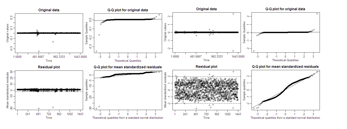
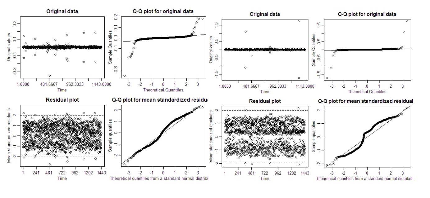
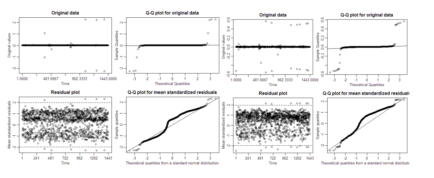
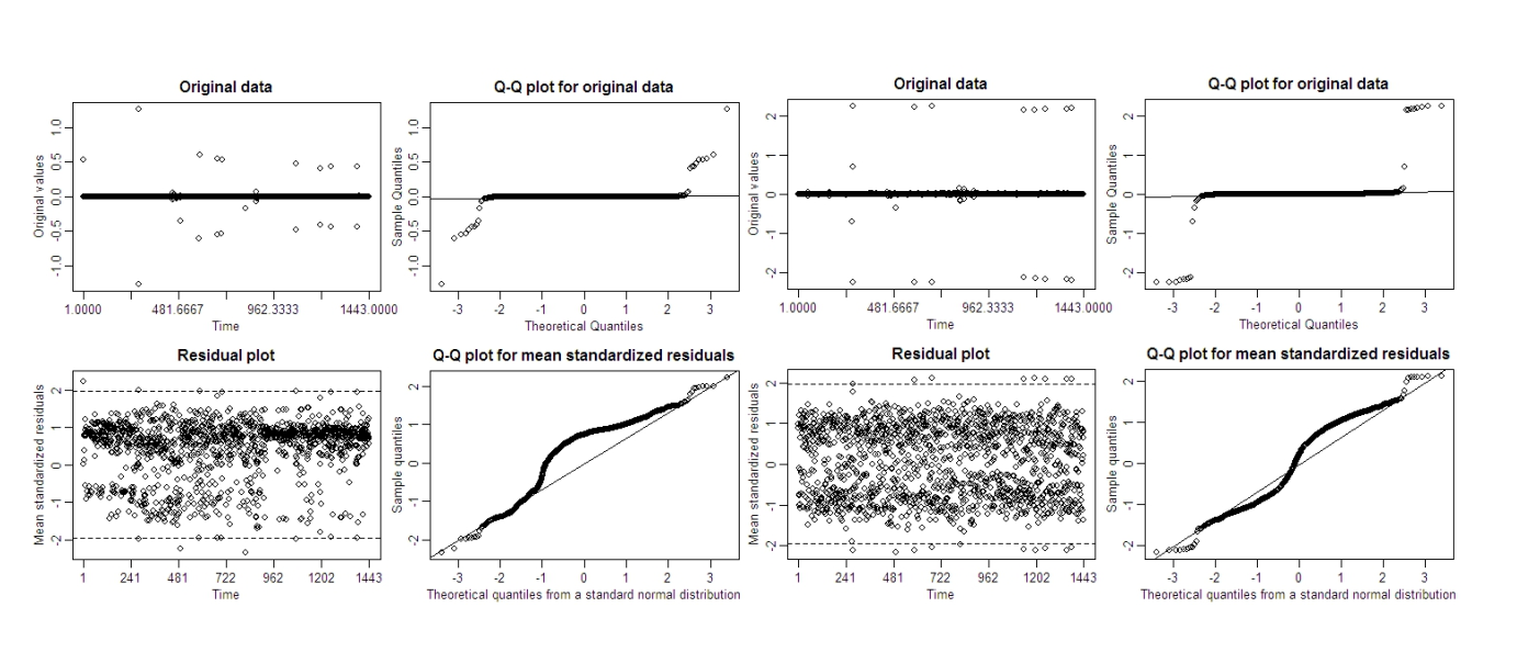
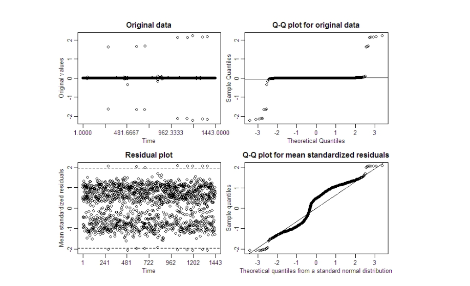
Figure 2. Residual Plots of the Naira-US Dollar and Naira-Pounds respectively

Figure 3. Residual Plots of the Naira-Euro and Naira-CFA respectively.

Figure 4. Residual Plots of the Naira-Yen and Naira-Swiss Franc respectively.

Figure 5. Residual Plots of the Naira-WAUA and Naira-RiyaL respectively.

Figure 6. Residual Plots of the Naira-Yuan and Naira-Danish Krone respectively.

Figure 7. Residual Plot of the Naira- SDR.

From the standardized mean residual plots for assessing the fitted models, the dashed lines in the bottom left panel indicate the 2.5% and 97.5% quantiles of the standard normal distribution of the range of rates clustered around the mean. The Q-Q plot for the mean standardized residuals revealed a clearing trait of bi-modality in the Naira-SDR, Naira-Danish Krone, Naira-WAUA, Naira-CFA, Naira-Euro, Naira-Pounds Sterling, and Naira-Swiss Franc while Naira-US Dollar, Naira-Riyal, and Naira-Yen unveiled a single modal for the currencies${^,}$ exchange series.

6. Conclusion

From the preceding, the Bayesian setting of Stochastic Volatility not only gave the circumstances of the fluctuation at quantile$^,$s (percentiles) levels of the latent autoregressive indexes but also the revealed stationarity processes of each of the rates$^,$ series via the prior$^,$s distributional mean and variance of the autoregressive coefficients. The posterior volatility estimates at 5%, 50%, and 95% quantiles of ${e^{\frac{\mu }{2}}}$ = (0.130041, 0.1502 and 0.1795) respectively for Naira-US Dollar exchange rates was the highest rates bartered fluctuation. The Naira-SDR exchange rate received a lesser up and rising rates with ${e^{\frac{\mu }{2}}}$ = (0.002, 0.0021, 0.0023) for 5%, 50%, and 95% quantiles. This might be due to low market trading of the reserve currency.

Author Contributions

All authors contributed equally to the writing of this paper. All authors read and approved the final manuscript.

Conflict of Interests

''The authors declare no conflict of interest.''

References

Markowitz, H. (1952). Portfolio Selection. The Journal of Finance 7(1), 77-91. [Google Scholor]
Wang, Q. Econ 762 Stochastic Volatility, 400060297, 2017. [Google Scholor]
Kastner, G. (2016). Dealing with Stochastic Volatility in Time Series Using the R Package Stochvol. Journal of Statistical Software, 69(5), 1-30. [Google Scholor]
Bos, C. S. (2012). Relating Stochastic Volatility Estimation Methods. In L Bauwens, C Hafner, S Laurent (eds.) Handbook of Volatility Models and Their Applications, John Wiley & Sons, 147 - 174. [Google Scholor]
Kim, S., Shephard, N., & Chib, S. (1998). Stochastic volatility: likelihood inference and comparison with ARCH models. The Review of Economic Studies, 65(3), 361-393. [Google Scholor]
Men, H. (2012). Bayesian Inference for Stochastic Volatility Models. Waterloo, Ontario, Canada. [Google Scholor]
Engle, R. F. (1982). Autoregressive conditional heteroscedasticity with estimates of the variance of United Kingdom inflation. Econometrica: Journal of the Econometric Society, 50(4), 987-1007. [Google Scholor]
Bollerslev, T. (1986). Generalized autoregressive conditional heteroskedasticity. Journal of Econometrics, 31(3), 307-327. [Google Scholor]
Cuervo, E. C., Achcar, J. A., & Barossi-Filho, M. (2014). New volatility models under a Bayesian perspective: a case study. Economia Aplicada, 18(2), 179-197. [Google Scholor]
Nelson, D. B. (1991). Conditional Heterocedasticity in asset returns: a New Approach. Econometrica, 59(2), 347 - 370, 1991. [Google Scholor]
Engle, R. F., & Ng, V. K. (1993). Measuring and testing the impact of news on volatility. The Journal of Finance, 48(5), 1749-1778. [Google Scholor]
Broto, C., & Ruiz, E. (2004). Estimation methods for stochastic volatility models: a survey. Journal of Economic Surveys, 18(5), 613-649. [Google Scholor]
Harvey, A. C., & Shephard, N. (1996). Estimation of an asymmetric stochastic volatility model for asset returns. Journal of Business & Economic Statistics, 14(4), 429-434. [Google Scholor]
Bauwens, L., Hafner, C. M., & Laurent, S. (2012). Handbook of volatility models and their applications (Vol. 3). John Wiley & Sons. [Google Scholor]
Taylor, S. J. (1982). Financial returns modelled by the product of two stochastic processes-a study of the daily sugar prices 1961-75. Time Series Analysis: Theory and Practice, 1, 203-226. [Google Scholor]
Szerszen, P. J. (2009). Bayesian analysis of stochastic volatility models with lévy jumps: application to risk analysis. Divisions of Research & Statistics and Monetary Affairs, Federal Reserve Board. [Google Scholor]
Nilsson, O. (2016). On Stochastic Volatility Models as an Alternative to GARCH Type Models. Department of Statistics, Uppsala University, Sweden. [Google Scholor]

\(\mu\)	Normal (Mean = -10, SD = 1)
\(\frac{{{\phi _{ + 1}}}}{2}\)	\(\beta\) (a= 20, b= 1.1)
\({\sigma ^2}\)	0.1 * Chis-squared (d.f = 1)