Magneto-squeezing flow and heat transfer analyses of third grade fluid between two disks embedded in a porous medium using Chebyshev spectral collocation method
The present study is based on the nonlinear analysis of unsteady magnetohydrodynamics squeezing flow and heat transfer of a third grade fluid between two parallel disks embedded in a porous medium under the influences of thermal radiation and temperature jump boundary conditions are studied using Chebyshev spectral collocation method. The results of the non-convectional numerical solutions verified with the results of numerical solutions using fifth-order Runge-Kutta Fehlberg-shooting method and also the results of homotopy analysis method as presented in literature. The parametric studies from the series solutions show that for a suction parameter greater than zero, the radial velocity of the lower disc increases while that of the upper disc decreases as a result of a corresponding increase in the viscosity of the fluid from the lower squeezing disc to the upper disc. An increasing magnetic field parameter, the radial velocity of the lower disc decreases while that of the upper disc increases. As the third-grade fluid parameter increases, there is a reduction in the fluid viscosity thereby increasing resistance between the fluid molecules. There is a recorded decrease in the fluid temperature profile as the Prandtl number increases due to decrease in the thermal diffusivity of the third-grade fluid. The results in this work can be used to advance the analysis and study of the behaviour of third grade fluid flow and heat transfer processes such as found in coal slurries, polymer solutions, textiles, ceramics, catalytic reactors, oil recovery applications etc.
The flows of non-Newtonian fluids between two plates are very important research interests in physics and engineering. Such flows are evident in moving pistons, catalytic reactors, flow inside syringes and nasogastric tubes, oil recovery applications, chocolate fillers, power transmission squeezed film, hydraulic lifts, compression, electric motors, injection modeling etc. The continuous wide areas of engineering, industrial and biological applications of fluid and heat transfer flow between two parallel discs or surfaces have inspired various researchers in recent times to critically study the problem. Considering the problem from heat and mass transfer analysis, Mustafa et al., [1] performed transient heat transfer analysis of squeezing fluid flow through two parallel surfaces. Hayat et al., [2] did a study on second grade fluid being squeezed by two parallel discs and presented with proper comparison the behaviour of the second-grade fluid considering or neglecting magnetic effect. In an attempt to solve the extension of Hayat et al., model considering suction and injection on magneto-hydrodynamic squeezing flow, Domairry and Aziz [3] used a semi-analytical method, homotopy perturbation method to obtain a symbolic solution for investigating and predicting the influence of suction and injection on magneto-hydrodynamic squeezing flow under standard conditions. A similar study was performed by Siddiqui et al., [4] using two parallel plates with the squeezing viscous fluid under transient condition. Immediately after that, Rashidi et al., [5] approached the problem using different analytical schemes. Incorporating nano-technology into the problem of squeezing flow, Khan and Aziz [6,7], investigated on the effect of natural convection on fluids with nano-particles. They extended their work on squeezing nanofluids by later considering porosity. A further study on squeezing nanofluid flow between two plates was perform by Kuznestov and Nield [8]. They investigated the boundary layer of the squeezing process by using natural convection principle of fluid flow to generate different governing models. Hashimi et al., [9] found the models interesting and obtained analytical solutions to the governing equations with the assumption of zero slip and zero temperature jump. The researchers mentioned above performed their interesting research based on the assumption of zero slip and zero temperature jump. However, these two annulled assumptions have to a reasonable extent influence on the processes in question. In other to provide an extension to the works of the above researchers as required, studies have been performed on squeezable fluids of different nano-particles sizes, different concentration, different stretching effect and different phases by taking slip into account [11,12,13,14,15]. The obtained model for the process were documented and proper parametric studies were performed to understand the process in general [16,17,18,19,20]. Past research works have presented magnetohydrodynamic fluid flow considering porous medium, nanofluid and some other factors capable of reshaping the squeezing process from idealization into actual [21,22,23,24,25,26,27]. In recent times, the flow and heat transfer characteristics of third grade nanofluid in pipes and in porous channel have been analyzed [28,29,30]. Since it has been established by Fosdick and Rajagopal [31] that third grade fluid gives different properties to those of fluids such as Newtonian and second grade fluids, Majhi and Nair [32] tried to manage the shearing stresses at the wall of a fluid flow process considering a third grade fluid as the working fluid. They compared their obtained results to the numerical solutions obtained by Massoudi and Christie [33] and an excellent agreement was reached by the two researchers. A third grade fluid with constant viscosity was considered by Yurusoy and Pakdemirli [34]. In order to verify their work with the available numerical solution of Vajrevelu et al., [35] for third grade fluid flow, they considered a governing equation with varying viscosity under no slip condition. The research work gave interesting results and found great application in rotary devices. Other studies on third grade fluids includes the fluctuating fluid flow by Hayat et al., [36], boundary layer analysis by Muhammet [37], heat transfer analysis by Yurusoy [38], entropy generation analysis by Pakdemirli et al., [39] and partial slip analysis by Sajid et al., [40]. Different schemes have also been employed to efficiently solve the resulting ordinary differential equations associated with squeezing fluid flow between two parallel surfaces as presented by [41,42,43,44,45,46,47].
Chebyshev spectral collocation method has demonstrated fast rate of convergence in the computation of nonlinear problems. It provides exponential convergence [48] which shows it superiority over other numerical methods such as finite element method (FEM) and the finite volume method (FVM) that provide linear convergence. Also, it has a very large converging speed over most of the commonly used numerical methods. It has been widely applied in computational fluid dynamics [49,50], electrodynamics [51] and magnetohydrodynamics [52,53] and other problems related to the solution of non-linear differential equations [54,55,56,57,58,59,]. It high level of accuracy to nonlinear differential equations has been well established [60,61,62,63]. However, to the best of the authors’ knowledge, this method has not been applied to the analysis of flow and heat transfer of most non-Newtonian fluid such as third grade fluid. Furthermore, the numerical study magnetohydrodynamic squeezing unsteady flow of third grade nanofluid between two parallel disks embedded in a porous medium under the influences of thermal radiation and temperature jump condition has not been considered and analyzed in literature. Therefore, in this work, nonlinear analysis of unsteady squeezing flow and heat transfer of a third grade fluid between two parallel disks embedded in a porous medium under the influences of thermal radiation and temperature jump boundary conditions is studied analytically and numerically using Chebyshev spectral collocation method. Also, parametric studies are carried out and the influences of various parameters on the flow and heat transfer processes are established.
2. Problem Formulation
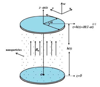
Consider an axisymmetrically flow of third grade fluid through two parallel disks as shown in Figure 1. The upper disk is moving towards the stationary lower disks under a uniform magnetic field strength applied perpendicular to disks as depicted in Figure 1. The fluid conducts electrical energy as it flows unsteadily under the influence of magnetic force field. It is assumed that the fluid structure is everywhere in thermodynamic equilibrium and the plate is maintained at constant temperature.
Figure 1. The squeezing flow of third grade fluid between parallel circular plate.
The Cauchy stress tensor, \(\tau \) for an incompressible homogeneous thermodynamically compatible third grade fluid is given by
where \(\tau \) is the stress tensor, \(\rho\) is the pressure, I is the identity tensor, \(\mu \) is the dynamic viscosity, \(I\) is the identity tensor, \(\alpha _{1} \),\(\alpha _{2} \),\(\beta _{1} \), \(\beta _{2} \) and \(\beta _{3} \) are the material constant and \(A_{1} \), \(A_{2} \) and \(A_{3} \) being the first, second and third Rivilin Erickson tensor which can be derived from
where \(V\) denotes velocity field, grad is the operator gradient and \(d/dt\) is the material time derivative. According to Fosdick and Rajagopal [31] motion of the fluid must be in accordance with the thermodynamic model (Clausius Duhem inequality must be satisfied). When the motions of the fluid are thermodynamically compatible, the Clausius-Duhem inequality and the assumption that the Helmholtz free energy is minimum when the fluid is locally at rest (stable) require that
Since \({\beta }_3>0\), the stress tensor can predict shear thickening as well as the normal stress. Velocity and temperature fields are:
\begin{equation}
\label{GrindEQ__5_}
V=(u(t,r,z),0,w(t,r,z))\text{ and }T=T(t,r,z),
\end{equation}
(5)
here \(u\) and \(w\) are the radial and axial components of velocity. From the above Equations (1-5), the algebraic forms of the conservation equations can be developed as
After substitution of Equations (9-12) into above momentum equations in Equations (7) and (8) and expansion of the resulting equations, one arrives at Equations (13) and (14)
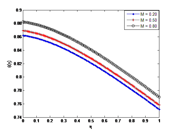
Figure 2. Influence of Hartman number on dimensionless.
Identically, it is established that the continuity equation is satisfied. Omitting the pressure terms from the momentum equations in Equations (13) and (14) and using the above transformations, one obtains
3. Chebyshev spectral collocation method for the solutions of the governing equations
It is obvious that Equations (17) and (18) are nonlinear partially coupled ordinary differential equation. Indisputably, it is very difficult if not impossible to develop exact analytical solutions for the equations. Therefore, we apply a numerical method, a spectral collocation method of the Chebyshev type to fluid flow and heat transfer equations. The method uses Chebyshev polynomials for expansion of the involving variables. The variables are expanded at the collocation points and then the derivatives of the at the collocation points are sought. After this, the expansions are substituted into the differential equations and the approximated solution in physical space are finally sought for.
In order to find approximate solution, which is a global Chebyshev polynomial of degree N defined on the interval \([-1,1]\), the interval is discretized by using collocation points to defined the Chebyshev nodes in \([-1,1]\), namely
The Chebyshev polynomials are defined on the finite interval \([-1,1]\). Therefore, to apply Chebyshev spectral method to the Equations (17) and (18), we make a suitable linear transformation and transform the physical domain \([-1,1]\) to Chebyshev computational domain
\([-1,1]\). We sample the unknown function w at the Chebyshev points to obtain the data vector \(w=\left[w\left(x_{o} \right),w\left(x_{1} \right),w\left(x_{2} \right),…w\left(x_{N} \right)\right]^{T} \). The next step is to find a Chebyshev polynomial P of degree N that interpolates the data \(\left(i.e.,\quad P\left(x_{j} \right)=w_{j} ,\; j=0,1,…N\right)\) and obtains the spectral derivative vector w by differentiating \(P\) and evaluating at the grid points \(\left(i.e.,\quad w_{j}^{‘} =P’\left(x_{j} \right)=w_{j} ,\; j=0,1,…N\right)\). This transforms the nonlinear differential equation into system nonlinear algebraic equations, which are solved by Newton’s iterative method starting with a initial guess.
With the aid of a suitable transformation, we map the physical domain \([0,1]\) to a computational domain \([-1,1]\) to facilitate our computations.
Equations (17) and (18) are transformed to the following equations,
And the boundary conditions in Equation (18) become
\begin{equation*} \label{GrindEQ__32_}
\; \tilde{f}\left(-1\right)=A,\quad \tilde{f}\left(1\right)=\frac{Sq}{2} ,\quad \sum _{j=0}^{N}d_{0}^{\left(1\right)} \tilde{f}\left(\eta _{j} \right)=1,\, \, \, \, \, \sum _{j=0}^{N}d_{N,j}^{\left(1\right)} \tilde{f}\left(\eta _{j} \right)=0,
\end{equation*}
\begin{equation*} \label{GrindEQ__33_}
\sum _{j=0}^{N}d_{N,j}^{\left(1\right)} \tilde{\theta }\left(\eta _{j} \right)=\Upsilon _{1} \left(\tilde{\theta }(-1)-1\right),{ \; }\sum _{j=0}^{N}d_{N,j}^{\left(1\right)} \tilde{\theta }\left(\eta _{j} \right)=-\Upsilon _{2} \tilde{\theta }(1)\quad
\end{equation*}
The above system of nonlinear algebraic equation contains \(3\)N-\(2\) equations for the unknown\(\tilde{f}\left(\eta _{j} \right),\; i=1,2,3,…,N\) and \(\tilde{\theta }\left(\eta _{j} \right),\; i=1,2,3,…,N-1\) is solved by Newton’s method.
4. Flow and heat transfer parameters of interests
Another set of important considerations in the analysis of fluid flow and heat transfer are skin friction coefficient and Nusselt number. The local skin friction coefficient at lower disk is
\begin{equation*} \label{GrindEQ__50_}
C_{f} =\frac{\tau _{w} |_{x=0} }{\frac{1}{2} \rho U_{w}^{2} },
\end{equation*}
while the local Nusselt number at the disk is
\begin{equation*} \label{GrindEQ__51_}
Nu=\frac{h(t)q_{w} }{K\left(T_{f} -T_{h} \right)} |_{z=0},
\end{equation*}
where wall heat flux is defined as:
\[q_{w} |_{z=0} =-K\frac{\partial T}{\partial z} |_{z=0} +q_{r} |_{z=0} .\]
Using the similarity variables in Equation (16) and the dimensionless parameters in Equation (21), one obtains the dimensionless forms of the local skin friction coefficient and Nusselt number as
\begin{equation*} \label{GrindEQ__52_}
C_{f} =\sqrt{2} Re^{-0.5} \left(\begin{array}{l} {2f”(0)+\alpha \left(3Sqf”(0)-2Af”'(0)+2f”(0)\right)} \\ {{ \; \; \; \; \; \; \; \; \; }-2\gamma f”(0)+\beta \left(\frac{Re}{4} f”’^{{}^{3} } (0)+6f”(0)\right)} \end{array}\right),
\end{equation*}
\begin{equation*} \label{GrindEQ__53_}
Nu=\left(1+Rd\right)\theta ‘(0).
\end{equation*}
5. Results and discussion
The results of homotopy perturbation method and the developed fifth-order Runge-Kutta Fehlberg method (RKFM) coupled with shooting method are presented in Table 1. Parametric studies are carried out and the influences of various parameters on the flow and heat transfer processes are established as shown in Figures 2-18.
Table 1. Numerical values of Nusselt number for different parameter.
RKFM
HAM
CSCM
\(\alpha\)
\(\gamma\)
\(\beta\)
Re
M
\(S_{q}\)
A
\(-Re^{\frac{1}{2}}C_{f}\)
\(-Re^{\frac{1}{2}}C_{f}\)
\(-Re^{\frac{1}{2}}C_{f}\)
0.01
0.10
0.10
1.00
0.40
1.00
0.01
3.88243
3.88243
3.88243
0.02
3.95950
3.95950
3.95950
0.03
4.03655
4.03655
4.03655
0.01
0.11
3.85249
3.85249
3.85249
0.12
3.82255
3.82255
3.82255
0.13
3.79260
3.79260
3.79260
0.10
0.20
4.63884
4.63884
4.63884
0.25
5.02298
5.02298
5.02298
0.29
5.33196
5.33196
5.33196
0.10
0.10
3.85868
3.85868
3.85868
0.20
3.86116
3.86116
3.86116
0.30
3.86368
3.86368
3.86368
1.00
0.50
3.90088
3.90088
3.90088
0.60
3.92337
3.92337
3.92337
0.70
3.94985
3.94985
3.94985
0.40
0.70
6.41631
6.41631
6.41631
0.75
6.00413
6.00413
6.00413
0.80
5.58953
5.58953
5.58953
1.00
0.02
4.06568
4.06568
4.06568
0.03
4.24817
4.24817
4.24817
0.04
4.42993
4.42993
4.42993
Table 2. Numerical values of Nusselt number for different parameter.
RKFM
HAM
CSCM
\(\alpha\)
\(\gamma\)
\(\beta\)
\(S_{q}\)<
\(P_{r}\)
\(E_{c}\)
\(\gamma_{1}\)
\(\gamma_{2}\)
Rd
Nu
Nu
Nu
0.01
0.10
0.10
1.00
0.10
0.10
0.20
0.20
0.20
0.092034
0.092034
0.092034
0.02
0.091945
0.091945
0.091945
0.03
0.091856
0.091856
0.091856
0.01
0.11
0.092149
0.092149
0.092149
0.12
0.092265
0.092265
0.092265
0.13
0.092380
0.092380
0.092380
0.10
0.20
0.088806
0.088806
0.088806
0.25
0.087186
0.087186
0.087186
0.29
0.085563
0.085563
0.085563
0.10
0.70
0.093319
0.093319
0.093319
0.75
0.092502
0.092502
0.092502
0.80
0.093528
0.093528
0.093528
1.00
0.11
0.090331
0.090331
0.090331
0.12
0.088628
0.088628
0.088628
0.13
0.086926
0.086926
0.086926
0.10
0.15
0.083306
0.083306
0.083306
0.25
0.065851
0.065851
0.065851
0.35
0.048396
0.048396
0.048396
0.10
0.30
0.108540
0.108540
0.108540
0.40
0.119230
0.119230
0.119230
0.50
0.126720
0.126720
0.126720
0.20
0.70
0.090240
0.090240
0.090240
0.80
0.092731
0.092731
0.092731
0.90
0.094174
0.094174
0.094174
0.20
0.30
0.101120
0.101120
0.101120
0.40
0.110210
0.110210
0.110210
0.50
0.119300
0.119300
0.119300
5.1. Influence of Hartman number and Squeezing parameter on dimensionless temperature profile
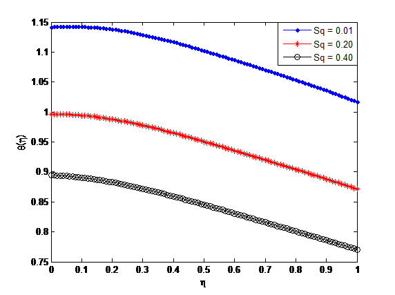
Figures 2 and 3 depict the influence of Hartman number and Squeezing parameter on dimensionless temperature profile. It is clear that as the Hartman number becomes large, it automatically raises the magnetic field as a result of an increase in the Lorentz force. This makes the temperature profile to increase as the Hartman number increases. Considering Figure 3, a rapid increase in the dimensionless temperature profile is noticed for a large value of squeezing parameter as a result of a driving compressive rotary force which generates a noticeable heating effect thereby increasing the temperature profile.
Figure 3. Influence of squeezing parameter on dimensionless.Figure 4. Influence of the first thermal Biot number on dimensionless temperature profile.
5.2. Influence of the thermal Biot number and Radiation term on dimensionless temperature profile
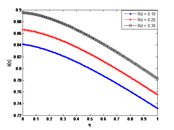
Figures 4-6 depict the influence of the thermal Biot number and Radiation term on dimensionless temperature profile. In Figures 4 and 5, the two thermal Biot number have opposing effect on the dimensionless temperature profile but the cooling effect generated by the first Biot number is more that the temperature rising effect obtained from the second even for the same range of values. As a result, these parameters can serve as a control for temperature monitoring. However, in Figure 6, as the radiation parameter increases, the dimensionless temperature profile increases. This is because, an increase in the radiation property causes a reduction in the absorptivity and consequently increases the rate of heat transfer to the third grade fluid.
Figure 5. Influence of the second thermal Biot number on dimensionless temperature profile.Figure 6. Influence of Radiation term on dimensionless temperature profile.Figure 7. Influence of \(\alpha\) on dimensionless velocity profile.
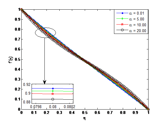
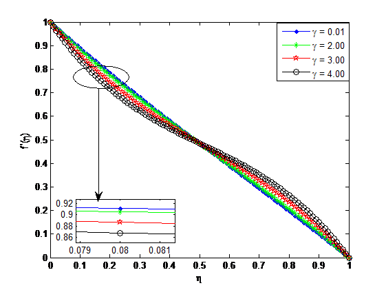
5.3. Influence of the third grade fluid parameters on dimensionless velocity profile
Figures 7-10 depict the influence of fluid flow parameters on dimensionless velocity profile. It is evident that an increase in the fluid flow parameters of the squeezing flow causes a corresponding increase in the fluid flow velocity. This is because the fluid flow parameters in question vary inversely with the viscosity of the fluid being squeezed. As these parameters increase, the viscosity of the fluid decreases and consequently increases the velocity of the fluid as the molecules of the squeezing flow are free to move with less restriction. These parameters can be used as a monitoring agent as they directly affect the viscosity of the third grade squeezing fluid.
Figure 8. Influence of \(\beta\) on dimensionless velocity profile.Figure 9. Influence of \(\gamma\) on dimensionless velocity profile.Figure 10. Better insight of the influence of \(\gamma\) on dimensionless velocity profile.
5.4. Influence of suction and squeezing parameters on dimensionless velocity profile
Figures 11 and 12 depict the influence of suction and squeezing parameters on dimensionless velocity profile. Figure 11 shows how the suction parameter affects the velocity of the squeezing discs for an increasing value of the fluid parameters. It is obvious that for a suction parameter greater than zero, the radial velocity of the lower disc increases while that of the upper disc decreases as a result of a corresponding increase in the viscosity of the third grade fluid from the lower squeezing disc to the upper disc. Figure 12 depicts the impact of the squeezing parameter on the fluid flow between the parallel discs. The figure shows that an increase in the squeezing parameter causes a corresponding increase in the squeezing rate. This is because as the squeezing parameter increases, the radial velocity of the squeezing discs increases there by generating a driving compressive rotary force on the fluid flowing between the two parallel discs.
Figure 11. Influence of suction term on dimensionless velocity profile.Figure 12. Influence of squeezing term on dimensionless velocity profile.
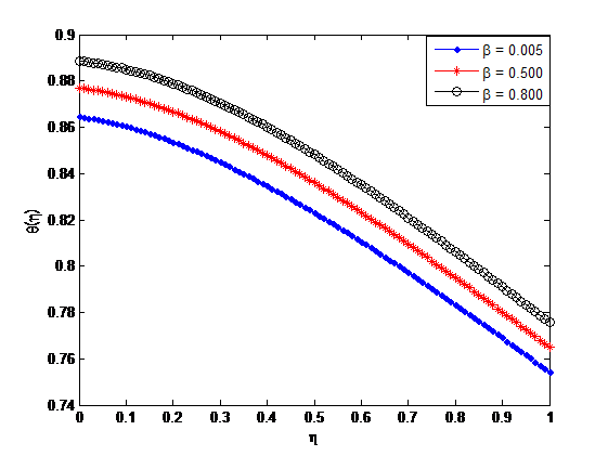
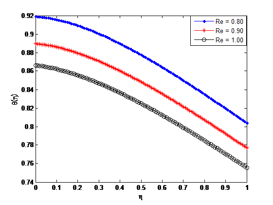
5.5. Influence of the third grade fluid parameter and Reynold’s number on dimensionless temperature profile
Figures 13 and 14 depict the influence of the third grade fluid parameter and Reynold’s number on dimensionless temperature profile. It has been ascertained that an increase in the third grade fluid parameter causes reduction in the fluid viscosity thereby increasing resistance between the fluid molecules. However, as the Reynold’s number associated with the third grade fluid increases, a decreasing effect is noticed in the dimensionless temperature profile. This is because there is a reduction in the convective capability of a high velocity fluid as compare to that with a moderate velocity.
Figure 13. Influence of the third grade fluid parameter on Dimensionless temperature profile.Figure 14. Influence of Reynold’s number on dimensionless Dimensionless temperature profile.
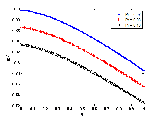
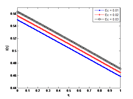
5.6. Influence of Prandtl and Eckert number on dimensionless temperature profile
Figures 15 and 16 depict the influence of Prandtl and Eckert number on dimensionless temperature profile. Figure 15 depicts a decrease in temperature profile as the Prandtl number increases. This is because an increase in the Prandtl number reduces thermal diffusivity thereby reducing the temperature profile. In Figures 16, Eckert number is observed to have a linear increasing property on the dimensionless temperature profile. This is because of the increase in the total kinetic energy of the fluid which correspondingly elevate the fluid temperature.
Figure 15. Influence of Prandtl number on dimensionless temperature profile.Figure 16. Influence of Eckert number on dimensionless temperature profile.
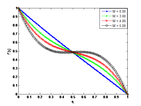
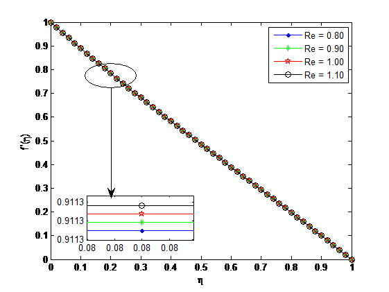
5.7. Influence of Hartman and Reynold’s number on dimensionless velocity profile
Figure 17. Influence of Hartman number on dimensionless velocity profile.Figure 18. Influence of Reynold’s number on dimensionless velocity profile.
Figures 17 and 18 depict the influence of Hartman number and Reynold’s number on dimensionless velocity profile. Figure 17 shows how the Hartman number affects the velocity of the squeezing discs for an increasing value of the fluid parameters. It is obvious that for a Hartman number greater than zero or for an increasing Hartman number, the radial velocity of the lower disc decreases while that of the upper disc increases as a result of a corresponding increase in the viscosity of the third grade fluid from the upper disc to the lower squeezing disc. As the Hartman number becomes large, it automatically raises the magnetic field as a result of a corresponding increase in the Lorentz force, hence decreases the flow velocity while increase in Reynold’s number increases the velocity of the fluid as shown in Figures 18.
6. Conclusion
In this study, nonlinear analysis of unsteady squeezing flow and heat transfer of a third grade nanofluid between two parallel disks embedded in a porous medium under the influences of thermal radiation and temperature jump boundary conditions were investigated. The developed flow and thermal models were solved numerically using Chebyshev spectral collocation method. Also, the influences of various flow and heat transfer parameters were investigated. Important significance of study includes the study of flow and heat transfer of third grade fluid as applied in energy conservation, coal slurries, polymer solutions, textiles, ceramics, catalytic reactors, oil recovery applications, friction reduction and micro mixing biological samples.
Nomenclature
A     Suction/injection parameter
B     magnetic field strength,Nm/A
\(c_{p}\)     specific heat capacity at constant pressure, J/kgK
\(c_{w}\)     specific heat capacity of the nanofluid, J/kgK
h     height of the flow, m
H     total distance between the two disks, m
\(k_{nf}\)    thermal conductivity of the nanofluid, W/mK
\(K_{p}\)     permeability of the porous medium, \(m^{2}\)
M     Hartmann number or magnetic field parameter
P     Pressure,\(N/m^{2}\)
Pr     Prandtl’s number
r     radius of the disk, m
Sq     Squeeze number
t     time, s
T     temperature, K
\(\mu_{f}\)     dynamic viscosity of the basefluid, Ns/\(m^{2}\)
\(\mu_{nf}\)     dynamic viscosity of the nanofluid, Ns/\(m^{2}\)
All authors contributed equally in writing of this paper. All authors read and approved the final manuscript.
Conflict of Interests
The authors declare no conflict of interest.
References
Mustafa, M., Hayat, T., & Obaidat, S. (2012). On heat and mass transfer in the unsteady squeezing flow between parallel plates. Meccanica, 47(7), 1581-1589.
[Google Scholor]
Hayat, T., Yousaf, A., Mustafa, M., & Obaidat, S. (2012). MHD squeezing flow of second-grade fluid between two parallel disks. International journal for numerical methods in fluids, 69(2), 399-410.
[Google Scholor]
Domairry, G., & Aziz, A. (2009). Approximate analysis of MHD squeeze flow between two parallel disks with suction or injection by homotopy perturbation method. Mathematical Problems in Engineering, 2009.[Google Scholor]
Siddiqui, A. M., Irum, S., & Ansari, A. R. (2008). Unsteady squeezing flow of a viscous MHD fluid between parallel plates, a solution using the homotopy perturbation method. Mathematical Modelling and Analysis, 13(4), 565-576.
[Google Scholor]
Rashidi, M. M., Shahmohamadi, H., & Dinarvand, S. (2008). Analytic approximate solutions for unsteady two-dimensional and axisymmetric squeezing flows between parallel plates. Mathematical Problems in Engineering, 2008.[Google Scholor]
Khan, W. A., & Aziz, A. (2011). Natural convection flow of a nanofluid over a vertical plate with uniform surface heat flux. International Journal of Thermal Sciences, 50(7), 1207-1214.
[Google Scholor]
Khan, W. A., & Aziz, A. (2011). Double-diffusive natural convective boundary layer flow in a porous medium saturated with a nanofluid over a vertical plate: Prescribed surface heat, solute and nanoparticle fluxes. International Journal of Thermal Sciences, 50(11), 2154-2160.
[Google Scholor]
Kuznetsov, A. V., & Nield, D. A. (2010). Natural convective boundary-layer flow of a nanofluid past a vertical plate. International Journal of Thermal Sciences, 49(2), 243-247.
[Google Scholor]
Hashmi, M. M., Hayat, T., & Alsaedi, A. (2012). On the analytic solutions for squeezing flow of nanofluid between parallel disks. Nonlinear Analysis: Modelling and Control, 17(4), 418-430.
[Google Scholor]
Navier, C. L. M. H. (1827). Sur les lois du mouvement des fluids, Mem. Acad. Roy. Sci. Inst. Fr, 6, 389-440.
[Google Scholor]
Choi, C. H., Westin, K. J. A., & Breuer, K. S. (2002, January). To slip or not to slip: Water flows in hydrophilic and hydrophobic microchannels. In ASME International Mechanical Engineering Congress and Exposition (Vol. 36487, pp. 557-564).
[Google Scholor]
Matthews, M. T., & Hill, J. M. (2007). Nano boundary layer equation with nonlinear Navier boundary condition. Journal of mathematical analysis and applications, 333(1), 381-400.
[Google Scholor]
Martin, M. J., & Boyd, I. D. (2006). Momentum and heat transfer in a laminar boundary layer with slip flow. Journal of thermophysics and heat transfer, 20(4), 710-719.
[Google Scholor]
Ariel, P. D. (2007). Axisymmetric flow due to a stretching sheet with partial slip. Computers & Mathematics with Applications, 54(7-8), 1169-1183. [Google Scholor]
Wang, C. Y. (2009). Analysis of viscous flow due to a stretching sheet with surface slip and suction. Nonlinear Analysis: Real World Applications, 10(1), 375-380.
[Google Scholor]
Yao, S., Fang, T., & Zhong, Y. (2011). Heat transfer of a generalized stretching/shrinking wall problem with convective boundary conditions. Communications in Nonlinear science and Numerical simulation, 16(2), 752-760.
[Google Scholor]
Kandasamy, R., Loganathan, P., & Arasu, P. P. (2011). Scaling group transformation for MHD boundary-layer flow of a nanofluid past a vertical stretching surface in the presence of suction/injection. Nuclear Engineering and Design, 241(6), 2053-2059.
[Google Scholor]
Makinde, O. D., & Aziz, A. (2011). Boundary layer flow of a nanofluid past a stretching sheet with a convective boundary condition. International Journal of Thermal Sciences, 50(7), 1326-1332.
[Google Scholor]
Uddin, M. J., Alginahi, Y., Bég, O. A., & Kabir, M. N. (2016). Numerical solutions for gyrotactic bioconvection in nanofluid-saturated porous media with Stefan blowing and multiple slip effects. Computers & Mathematics with Applications, 72(10), 2562-2581.
[Google Scholor]
Uddin, M. J., Kabir, M. N., & Alginahi, Y. M. (2015). Lie group analysis and numerical solution of magnetohydrodynamic free convective slip flow of micropolar fluid over a moving plate with heat transfer. Computers & Mathematics with Applications, 70(5), 846-856.
[Google Scholor]
Raju, K. V. S., Reddy, T. S., Raju, M. C., Narayana, P. S., & Venkataramana, S. (2014). MHD convective flow through porous medium in a horizontal channel with insulated and impermeable bottom wall in the presence of viscous dissipation and Joule heating. Ain Shams Engineering Journal, 5(2), 543-551. [Google Scholor]
Bühler, L., Mistrangelo, C., & Najuch, T. (2015). Magnetohydrodynamic flows in model porous structures. Fusion Engineering and Design, 98, 1239-1243.
[Google Scholor]
Geindreau, C., & Auriault, J. L. (2001). Magnetohydrodynamic flow through porous media. Comptes Rendus de l’Académie des Sciences-Series IIB-Mechanics, 329(6), 445-450.
[Google Scholor]
Falade, J. A., Ukaegbu, J. C., Egere, A. C., & Adesanya, S. O. (2017). MHD oscillatory flow through a porous channel saturated with porous medium. Alexandria engineering journal, 56(1), 147-152.
[Google Scholor]
Pattnaik, J. R., Dash, G. C., & Singh, S. (2017). Radiation and mass transfer effects on MHD flow through porous medium past an exponentially accelerated inclined plate with variable temperature. Ain Shams Engineering Journal, 8(1), 67-75.
[Google Scholor]
Ali, F., Khan, I., Ul Haq, S., & Shafie, S. (2013). Influence of thermal radiation on unsteady free convection MHD flow of Brinkman type fluid in a porous medium with Newtonian heating. Mathematical Problems in Engineering, 2013.[Google Scholor]
Khan, A., Khan, I., Ali, F., & Shafie, S. (2014). Effects of wall shear stress on MHD conjugate flow over an inclined plate in a porous medium with ramped wall temperature. Mathematical Problems in Engineering, 2014.[Google Scholor]
Ogunmola, B. Y., Akinshilo, A. T., & Sobamowo, M. G. (2016). Perturbation solutions for Hagen-Poiseuille flow and heat transfer of third grade fluid with temperature-dependent viscosities and internal heat generation. International Journal of Engineering Mathematics, 8915745, 2016.
[Google Scholor]
Sobamowo, G., Akinshilo, A., Yinusa, A., & Adedibu, O. (2018). Nonlinear slip effects on pipe flow and heat transfer of third grade fluid with nonlinear temperature-dependent viscosities and internal heat generation. Software Eng, 6(3), 69-88.
[Google Scholor]
Akinshilo, A. T., & Sobamowo, G. M. (2017). Perturbation solutions for the study of MHD blood as a third grade nanofluid transporting gold nanoparticles through a porous channel. Journal of Applied and computational mechanics, 3(2), 103-113.
[Google Scholor]
Fosdick, R. L., & Rajagopal, K. R. (1980). Thermodynamics and stability of fluids of third grade. Proceedings of the Royal Society of London. A. Mathematical and Physical Sciences, 369(1738), 351-377.
[Google Scholor]
Majhi, S. N., & Nair, V. R. (1994). Flow of a third grade fluid over a sternosed tubes. Indian national science academy, 60(3), 535.
[Google Scholor]
Massoudi, M., & Christie, I. (1995). Effects of variable viscosity and viscous dissipation on the flow of a third grade fluid in a pipe. International Journal of Non-Linear Mechanics, 30(5), 687-699.
[Google Scholor]
Yürüsoy, M., & Pakdemirli, M. (2002). Approximate analytical solutions for the flow of a third-grade fluid in a pipe. International Journal of Non-Linear Mechanics, 37(2), 187-195.
[Google Scholor]
Vajravelu, K., Cannon, J. R., Rollins, D., & Leto, J. (2002). On solutions of some non-linear differential equations arising in third grade fluid flows. International journal of engineering science, 40(16), 1791-1805.
[Google Scholor]
Hayat, T., Nadeem, S., Asghar, S., & Siddiqui, A. M. (2001). Fluctuating flow of a third-grade fluid on a porous plate in a rotating medium. International Journal of Non-Linear Mechanics, 36(6), 901-916.
[Google Scholor]
Yürüsoy, M. (2003). Similarity solutions to boundary layer equations for third-grade non-Newtonian fluid in special coordinate system. Journal of theoretical and applied mechanics, 41(4), 775-787.
[Google Scholor]
Yürüsoy, M. (2004). Flow of a third grade fluid between concentric circular cylinders. Mathematical and Computational Applications, 9(1), 11-17. [Google Scholor]
Pakdemirli, M., & Yilbas, B. S. (2006). Entropy generation for pipe flow of a third grade fluid with Vogel model viscosity. International Journal of Non-Linear Mechanics, 41(3), 432-437.
[Google Scholor]
Sajid, M., Mahmood, R., & Hayat, T. (2008). Finite element solution for flow of a third grade fluid past a horizontal porous plate with partial slip. Computers & Mathematics with Applications, 56(5), 1236-1244.
[Google Scholor]
R. Elahi, T. Hayat, F. M. Mahomed and S. Asghar. Effects of slip on the nonlinear flow of the third grade fluid, Journal of the nonlinear analysis, volume 11, (2010) 139-146.
[Google Scholor]
Jayeoba, O. J., & Okoya, S. S. (2012). Approximate analytical solutions for pipe flow of a third grade fluid with variable models of viscosities and heat generation/absorption. Journal of the Nigerian mathematical society, 31, 207-227.
[Google Scholor]
Abbasbandy, S., Hayat, T., Ellahi, R., & Asghar, S. (2009). Numerical results of a flow in a third grade fluid between two porous walls. Zeitschrift für Naturforschung A, 64(1-2), 59-64.
[Google Scholor]
Nayak, I., Nayak, A. K., & Padhy, S. (2012). Numerical solution for the flow and heat transfer of a third grade fluid past a porous vertical plate. advanced studies theoretical physics, 6(13), 615-625.
[Google Scholor]
Aiyesimi, Y. M., Okedayo, G. T., & Lawal, O. W. (2013). Unsteady magnetohydrodynamic (MHD) thin film flow of a third grade fluid with heat transfer and no slip boundary condition down an inclined plane. International journal of physical sciences, 8(19), 946-955.
[Google Scholor]
Ogunsola, A. W., & Peter, B. A. (2014). Effect of variable viscosity on third grade fluid flow over a radiative surface with Arrhenius reaction. International journal of pure and applied sciences and technology, 22(1), 1.
[Google Scholor]
Yürüsoy, M., M. Pakdemirli, and B. S. Yilbas. “Perturbation solution for a third-grade fluid flowing between parallel plates.” Proceedings of the Institution of Mechanical Engineers, Part C: Journal of Mechanical Engineering Science 222, no. 4 (2008): 653-656.
[Google Scholor]
Gottlieb, D., & Orszag, S. A. (1977). Numerical analysis of spectral methods: theory and applications. Society for Industrial and Applied Mathematics.
[Google Scholor]
Canuto, C., Hussaini, M. Y., Quarteroni, A., & Zang, T. A. (1988). Spectral Methods in Fluid Dynamics (No. BOOK). Springer.
[Google Scholor]
Peyret, R. (2002). Spectral Methods for Incompressible Viscous Flow (Vol. 148). Springer Science & Business Media.
[Google Scholor]
Ben Belgacem, F., & Grundmann, M. (1998). Approximation of the wave and electromagnetic diffusion equations by spectral method. SIAM Journal on Scientific Computing, 20(1), 13-32.
[Google Scholor]
Shan, X., Montgomery, D., & Chen, H. (1991). Nonlinear magnetohydrodynamics by Galerkin-method computation. Physical Review A, 44(10), 6800. [Google Scholor]
Shan, X., & Montgomery, D. (1994). Magnetohydrodynamic stabilization through rotation. Physical review letters, 73(12), 1624.
[Google Scholor]
Wang, J. P. (2001). Fundamental problems in spectral methods and finite spectral method. Acta Aerodynamica Sinica, 19(2), 161-171.
[Google Scholor]
Elbarbary, E. M., & El-Kady, M. (2003). Chebyshev finite difference approximation for the boundary value problems. Applied Mathematics and Computation, 139(2-3), 513-523.
[Google Scholor]
Huang, Z. J., & Zhu, Z. J. (2009). Chebyshev spectral collocation method for solution of Burgers’ equation and laminar natural convection in two-dimensional cavities. Bachelor Thesis, University of Science and Technology of China, Hefei.[Google Scholor]
Eldabe, N. T., & Ouaf, M. E. (2006). Chebyshev finite difference method for heat and mass transfer in a hydromagnetic flow of a micropolar fluid past a stretching surface with Ohmic heating and viscous dissipation. Applied Mathematics and Computation, 177(2), 561-571.
[Google Scholor]
Khater, A. H., Temsah, R. S., & Hassan, M. (2008). A Chebyshev spectral collocation method for solving Burgers’-type equations. Journal of Computational and Applied Mathematics, 222(2), 333-350.
[Google Scholor]
Canuto, C., Hussaini, M. Y., Quarteroni, A., & Zang, T. A. (1988). Spectral Methods in Fluid Dynamics (No. BOOK). Springer.
[Google Scholor]
Doha, E. H., & Bhrawy, A. H. (2008). Efficient spectral-Galerkin algorithms for direct solution of fourth-order differential equations using Jacobi polynomials. Applied Numerical Mathematics, 58(8), 1224-1244.
[Google Scholor]
Doha, E. H., & Bhrawy, A. H. (2009). A Jacobi spectral Galerkin method for the integrated forms of fourth-order elliptic differential equations. Numerical Methods for Partial Differential Equations: An International Journal, 25(3), 712-739.
[Google Scholor]
Doha, E. H., Bhrawy, A. H., & Hafez, R. M. (2011). A Jacobi–Jacobi dual-Petrov–Galerkin method for third-and fifth-order differential equations. Mathematical and Computer Modelling, 53(9-10), 1820-1832.
[Google Scholor]
Doha, E. H., Bhrawy, A. H., & Ezz-Eldien, S. S. (2011). Efficient Chebyshev spectral methods for solving multi-term fractional orders differential equations. Applied Mathematical Modelling, 35(12), 5662-5672.
[Google Scholor]
Hayat, T., Nazar, H., Imtiaz, M., Alsaedi, A., & Ayub, M. (2017). Axisymmetric squeezing flow of third grade fluid in presence of convective conditions. Chinese Journal of Physics, 55(3), 738-754.
[Google Scholor]