Solving some variants of vehicle routing problem with Branch-and-cut and Column generation algorithms

1. Introduction

The cost of transportation of goods and services is one of the major challenges people face in their daily activities. This area has raised concern in todays society. A large sum of money is spent daily on fuel, goods and service delivery, equipment maintenance and so on [1]. This is where the knowledge and technique of Operations Research (OR) comes to play. If the available resources is known, one can employ the techniques of OR. According to [2], the use of computerized techniques in solving transportation problem most times often leads to about \(5% -20%\) savings on transportation cost. Therefore, planning of distribution process, research and studying OR-techniques is worthwhile and will save some transportation cost.

The Vehicle Routing Problem (VRP) has been a problem for several decades and one of the most studied problem in logistics engineering, applied mathematics and computer science, and which is described as finding optimal routes for a fleet of vehicles to serve some scattered customers from depot [3]. VRP have several variants which includes:

• Travelling Salesman Problem (TSP) [4],
• Capacitated Vehicle Routing Problem (CVRP) [5],
• Periodic Vehicle Routing Problem (PVRP) [6],
• Vehicle Routing Problem with Time Windows (VRPTW) [7],
• Vehicle Routing Problem with Skills Sets (VRPSS) [8],
• Vehicle Routing Problem with Pickup and Devlivery (VRPPD)

and so on.

The VRP is a combinatorial optimization and integer programming problem which finds optimal path in order to deliver goods and services to a finite set of customers.

The Travelling Salesman Problem (TSP) is one of the variant of Vehicle Routing Problem (VRP) which is a classical and widely studied problem in combinatorial optimization [9]. TSP has been studied in Operations Research (OR), engineering and computer science since \(1950\)s and several techniques been developed to solve this kind of problem. TSP describes a salesman who must travel through \(n\) cities. The order of visiting the cities is not of importance, as long as the salesman visit every city exactly once and return to the starting city [10]. The cities are connected to one another through a weighted link.

CVRP is another variant of VRP involves vehicles with limited carrying capacity of goods and these goods must be delivered. In CVRP, the major factors we consider are the customers demands, number of vehicles availabe and the vehicle capacity. The objective is to find optimal route such that each and every customer is served once and every vehicle is loaded according to its capacity and not more [1]. The first article was introduced by [11], which was related to the concept of vehicle routing problem by trying to solve the truck dispatching problem with the objective of finding optimal supply-technique from the bulk terminal to the large number of service stations. [12] implemented the branch and cut algorithm to solve a large scale traveling salesman problem where the problem has to be solved many times in branch and cut algorithm before a solution to the TSP was obtained. Using large scale instances of the TSP, a substantial portion of the execution time of the entire branch and cut algorithm is spent in linear program optimiser. In their work, they constructed a full implementation of branch and cut algorithm, utilising the special structure. However, all of the refinements discussed in [13] are not implemented. Column Generation (CG), an exact approach for solving VRP was used and reported successful in solving VRPTW [14,15]. With its success, many researchers perform their further research with this technique. [16] proposed and used CG technique to solve the Heterogeneous Fleet Vehicle Routing Problem (HVRP). Applications of Vehicle Routing Problem cut across several areas which includes; Courier service [17], realtime delivery of customers demand [18], milk runs dispatching system in real time [19] and milk collection problem [20].

The goal of this paper is to solve TSP and CVRP using branch-and-cut and column generation algorithms, respectively. We shall use methods that will give us optimal routes for each of these considered variants.

2.Formulations and methods

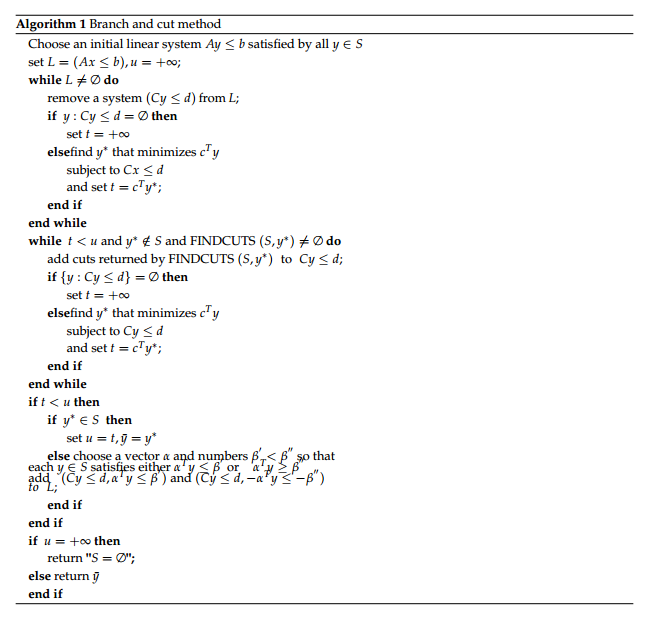
A Linear programming (LP) problem is a problem that is to maximize or minimize a linear function subject to specified linear equality or inequality constraints. A general form of an LP program is given as follows.

where \(x_{1}\), \(x_{2}\), ..., \(x_{n}\) are the variables and the remaining elements are input data from the problem. Also, \(l_{1}\), \(l_{2}\) ... \(l_{n}\) can be assigned the value of \(-\infty\) and \(u_{1}\), \(u_{2}\), ...,, \(u_{n}\) can be also be assigned the value \(+\infty\). Rewriting Equation (1) in matrix notation we have, $$A = \begin{pmatrix} a_{11}& a_{12} & \dots & a_{1n} \\ a_{21}& a_{21} & \dots & a_{2n} \\ \vdots & & & \\ a_{m1} & a_{m2} & \dots &a_{mn} \end{pmatrix} $$ and vectors $$(x =\begin{pmatrix} x_{1} \\ x_{2}\\ \dots\\ x_{n} \end{pmatrix},\hspace{.4cm} c =\begin{pmatrix} c_{1} \\ c_{2}\\ \dots\\ c_{n} \end{pmatrix}, \hspace{.4cm} b =\begin{pmatrix} b_{1} \\ b_{2}\\ \dots\\ b_{n} \end{pmatrix},$$ $$l =\begin{pmatrix} l_{1} \\ l_{2}\\ \dots\\ l_{n} \end{pmatrix}, \hspace{.4cm} u =\begin{pmatrix} u_{1} \\ u_{2}\\ \dots\\ u_{n} \end{pmatrix},$$ The general LP problem can be written as: where \(A\) is a matrix which is called the constraint matrix, \(c^{T}\) is the transpose of the \(c-\)vector. Vector \(b\) is a right hand side vector, vectors \(l\) and \(u\) are the lower and upper bounds; \(c^{T}x\) is the objective function. A feasible solution to the LP problem is an assignment of values \(x\) that satisfies all the constraints. An optimal solution \(x^{*}\) is a feasible solution such that \(c^{T}x^{*} \geq c^{T} \overset{-}{x}\) for all other feasible solutions \(\overset{-}{x}\) [24].

Definition 1. Given a system \(Ax = b\) of \(n\) linear equations in \(m\) variables, for \(m \ge n\). A basic solution to \(Ax = b\) is obtained by setting variables \(n - m = 0\) and solving for the values of the remaining \(m\) variables. This assumes that setting the \(n - m = 0\) produce unique values for the remaining \(m\) variables or, equivalently, the columns for the remaining \(m\) variables are linearly independent [24].

Definition 2. Any basic solution to (1) in which all variables are nonnegative is a Basic Feasible Solution(bfs) [24].

Theorem 3. (Extreme point [24]) A point in the feasible region of an LP is an extreme point if and only if it is a basic feasible solution to the LP.

Theorem 4. (Direction of unboundedness [24]) Consider an LP in standard form, having a bfs \(b_1, b_2, \dots, b_{k}\). Any point \(x\) in the LP's feasible region may be written in the form $$x = d + \sum_{i=1}^{i=k}\sigma_{i}b_{i} $$ where \(d\) is \(0\) or a direction of unboundedness and \(\sum_{i=1}^{i=k}\sigma_{i} = 1\) and \(\sigma_{i} \ge 0.\)

Theorem 5.(Optimal bfs [24]) Consider an LP with objective function max \(cx\) and constraints Ax = b. Suppose this LP has an optimal solution. We now sketch a proof of the fact that the LP has an optimal bfs. If an LP has an optimal solution, then it has an optimal bfs.

Proof. Let \(x\) be an optimal solution to our LP in (l). Because \(x\) is feasible, Theorem (4) tells us that we may write \(x = d + \sum_{i=1}^{i=k}\sigma_{i}b_{i}\), where \(d\) is \(0\) or a direction of unboundedness and \(\sum_{i=1}^{i=k}\sigma_{i} = 1\) and \(\sigma_{i} \ge 0.\) If \(cd > 0\), then for any \(k > 0\), \(kd + \sum_{i=1}^{i=k}\sigma_{i}b_{i}\) is feasible, and as \(k\) becomes larger and larger, the objective function value approaches \(\infty\). This contradicts the fact that the LP has an optimal solution. If \(cd < 0\), then the feasible point \(\sum_{i=1}^{i=k}\sigma_{i}b_{i}\) has a larger objective function value than \(x\). This contradicts the optimality of \(x\). In short, we have shown that if \(x\) is optimal, then \(cd = 0\). Now the objective function value for \(x\) is given by $$cx = cd + \sum_{i=1}^{i=k}\sigma_{i}cb_{i} = \sum_{i=1}^{i=k}\sigma_{i}cb_{i}.$$ Suppose that \(b_1\) is the bfs with largest objective function value. Because \(\sum_{i=1}^{i=k}\sigma_{i} = 1\) and \(\sigma_{i} \ge 0,\) so $$cb_1 \ge cx.$$ Because \(x\) is optimal, this shows that \(b_1\) is also optimal, and the LP does indeed have an optimal bfs.

2.1.Mathematical formulation of TSP Using ILP

There are several mathematical formulations for TSP [21]. Employing a variety of constraints that enforce the requirements of the problem in order to demonstrate how such a formulation is used in the comparative analysis as follows: given a complete graph \(G = (V,E)\) with \(\vert V \vert = n\) and \(\vert E \vert = m = \frac{n(n-1)}{2}\), and nonnegative cost of distance travelled, \( d_{ij}\), containing each vertex exactly once. Introducing binary variable \( y_{ij}\) for the possible inclusion of any edge \( (i,j) \in E \) in the tour we get the following classical ILP formulation; recall from previous section, since we can travel from one city to another, the graph is complete. That is to say, there is an link/edge between every pair of nodes. For each edge in the graph, we associate a binary variable as follows $$y_{ij} = \begin{cases} 1 \hspace{0.3cm} \text{if edge} \hspace{0.3cm} (i,j) \in \text{E is in tour } \\ 0 \hspace{0.3cm} \text{Otherwise} \end{cases}$$ and other nomenclatures are given as

• \(G=(V,E)\) represents a complete graph \(G\)
.
• \(V = \{v_1, v_2, \dots, v_n\}\); denotes set of cities.
• \(E = \{(v_{i}, v_{j}), v_0 \le i,j \le m \} \) edges between \(V\)
.
• \(d_{ij} = c:\) is the nonnegative cost-matrix of distance travel.
• Decision variable is defined as: \( y_{ij} = \begin{cases} 1 \hspace{0.3cm} \text{if edge} \hspace{0.3cm} (i,j) \in E\text{ is in tour } \\ 0 \hspace{0.3cm} \text{Otherwise} \end{cases} \)
• \(y^{*}\) is the optimal solution.
• \(\vert \vert . \vert \vert_{2}\) is euclidean norm.
• \(x\) represent sequence of cities.

Also since the edges are undirected, it suffices to include only edges with \( i < j \) in the model. Furthermore, since we are minimizing the total distance travelled during the tour, so we calculate \( d_{ij}\) between each pair of nodes \(i\) and \(j\). So the total distance travelled is the sum of all the distances of the edges which are included in the tour as follows.

Since the tour can only pass through each city exactly once, then each node in the graph should have exactly one incoming and one outgoing edge. i.e., for every \(i\) node, exactly two of \(y_{ij}\) binary variables should be equal to \(2\), and we write it as follows:

Furthermore, eliminating sub tours that might arise from the above constraint, we add the following constraints:

This constraints require that for each proper (non-empty) subset of the set of cities \(V\), the number of edges between the nodes of \(S\) must be at most \(\vert S \vert - 1.\) Therefore, the final integer linear problem of our TSP formulation is as follows:

\begin{equation*} Min \sum_{{(i,j) \in E }} d_{ij} y_{ij} \end{equation*} Subject to: \begin{equation*} \sum_{j \in V } y_{ij} = 2 \, \, \forall i \in V, \end{equation*} and if the set of cities \(V\) is of size \(n\) , then there are \( 2^{n} -2 \) subset of \(S\) of \(V\), excluding \( S=V \) and \( S = \emptyset\). Where Equation (3) defines the objective function, (4) is the degree equation for each vertex, (5) are the sub tour elimination constraints (SEC), which forbid solution consisting of several disconnected tours, and (6) defines the integrality constraints. Also note that some of the SEC are redundant: for the vertex set \( S \subset V, S \neq \emptyset\), and \( S^{'} = V \backslash S \) we get pairs of SEC both enforcing the connection of \( S\) and \( S^{'} \).

We used branch-and-cut algorithm given in [1] to solve TSP.

2.2.Mathematical formulation of CVRP

All vehicles will originate and end at the depot, while each of the customer is visited exactly once. Suppose we have a graph \(G=(\mathcal{V}, \mathcal{E})\), where \(\mathcal{V}, \mathcal{E}\) represent the sets of nodes and weighted edges respectively, let us define the following:

• \(\mathcal{C} = \{1, 2,\dots, m\}\): represent the set of \(m\)-customers to be considered.
• \(\mathcal{V} = \{{v_{0}},{v_{1}}, \dots, {v_{m}},{v_{m+1}}\}\) is the set of vertices in \(G\). The vertices \(v_{0}= v_{m+1}\) represent the depot, and \(\{{v_{1}},\dots,{v_{m}}\}\) represent customers nodes.
• \(\mathcal{E} = \{({v_{i}}, {v_{j}}) \hspace{.2cm} \vert \hspace{.2cm} 0 \le i,j \le m, \hspace{.2cm}i\ne j \}\) is a set of \(\vert \mathcal{V} \vert \ast (\vert \mathcal{V} \vert - 1)\) directed routes/edges between the vertices. If in both directions the distance between two vertices are identical, we then add the \((i < j)\) restriction.
• K: denote the fleet of available vehicles in a single depot. All vehicles considered are homogeneous.i.e., equal capacities. We have \(n\)-vehicles.
• Q: is the maximum capacity of a vehicle, which limits the number of customers to be visited before returning to the depot.
• C \(= (c_{ij})\) is the cost of traveling from nodes \(i\) to \(j\). and \(c_{ij}\ge 0\) is the corresponding distance of edges \((v_{i},v_{j})\), the diagonal of the matrix.i.e., \(c_{ii} = 0\) always. Depending on whether the VRP variant in consideration is symmetric or not, \(c_{ij} = c_{ji}\). The triangle inequality is assumed to hold generally.i.e., \(c_{ij} \le c_{ik}+c_{kj}\) and \((0 \le i,j,k \le m)\).
• \(R_i = (v_{0}^{i}, v_{1}^{i},v_{2}^{i}, v_{3}^{i} \dots, v_{k_i}^{i}, v_{k_{i+1}}^{i})\) is a vector of the route of vehicle \(i\) which start and end at the depot, with \(v_{0}^{i} = v_{k_{i+1}}^{i} = v_{0}, v_{j}^{i} \ne v_{\ell}^{i}, 0 \le j < \ell \le k_i\), and \(k_i\) is the length of route \(R_i\).
• \(\mathcal{S} = \{R_1,\dots, R_n\}\) is the set of route which represent the VRP solution instance.
• C\((R_{i}) = \sum_{j=0}^{k_i}\) C\((v_{j}^{i}, v_{j+1}^{i})\), the cost of route \(R_i\).
• C\(\mathcal{(S)} = \sum_{i=1}^{n}\) C\((R_i)\) is the total cost of solution \(\mathcal{S}\) which satisfies;

In order to serve each customer once, the route vectors is treated here as a set. The goal of the VRP is to minimize the C\(\mathcal{(S)}\) on the graph \(\mathcal{G}=(\mathcal{V},\mathcal{E})\).

Let \(\mathcal{G}\) is the graph which contains \(\vert \mathcal{E} \vert +2\) vertices, and the customers ranges from \((1,2,\dots, m)\). The starting and returning depots are denoted by \(0\) and \(m+1\) respectively. Earlier in this section, we introduced the vehicle routing problem which we have now defined. However, the problem is not all about visiting the customers, there is more to their demands. In the following definitions, we shall specify these additional demands of the customers:

• demand: \(d = (d_0, \dots, d_m, d_{m+1})\) with \(d_i> 0\) and \(m\) is the total number of customers which is a vector of the demands of customer, the demand of the depot is denoted by \(d_0\), \(d_0 = d_{m+1} = 0\) always.
• Let us define our decision variable: \(x_{ijk} = \left\{ \begin{array}{rcl} 1 & \mbox{iff vehicle \(k\) moves from node \(i\) to \(j\)} \\ \\ 0 & \mbox{otherwise.} \end{array}\right.\)
• q\(_{j}\) is the quantity of demand at node \(j\)

The problem definition will be based on the following assumptions:

• The capacity constraints of all the vehicles are observed.
• Each customer can be served by only one vehicle.
• Each and every route starts at vertex \(0\) and ends at vertex \((m+1)\).

The mathematical formulation of Capacitated Vehicle Routing Problem is stated below. We start with the objective function; which minimize the total travel cost by vehicle. This function is subjected to several constraints. subjected to: restrict each customer to be visited and served by only one vehicle. constraints (9), (10) and (11) ensure that each and every vehicle must originate from starting depot \(0\), pass through various destinations of demands and return to end depot \(m+1\). constraints (12) and (13) ensures the capacity constraint is observed. and constraint (14) indicate integrality constraints.

Note that subtours are avoided in the solution with constraint (12) that is, cycling paths which do not pass through the depot. Advantage of having constraints (12) and (13) in terms of our customers in this problem is that the formulation has a polynomial number of constraints.

2.2.1.Column generation

We shall solve this formulation using the column generation technique. A brief explanation of this technique is as follow:

• Restricted Master Problem: The Restricted Master Problem (RMP) is a set-partitioning problem. Some routes have the potential to improve the objective function, the RMP considers these paths which were added to the set of routes due to their potential to improve the objective function. The advantage of this technique is, only routes with high potential are added to the set of routes. Set partitioning problem has been considered because it is flexible with the objective function and its constraints. This approach allows the adding of constraints and this has an impact on the existing routes. This constraint- adding characteristics, makes set-partitioning problem more flexible than several other approaches[22] . When solving RMP (using simplex algorithm (2)), a dual value is assigned to each customer, this assigned value corresponds to how much we can improve the total solution by adding better routes including this customer.
• Pricing Problem: The second part of CG is the pricing-problem which is a sub-problem following the RMP to identify and generate new routes and column that will enter the set of routes (variables) in the RMP. The RMP assigns dual values to customers, which assists to identify new routes with potential to improve the objective function. The new routes generated from pricing-problem are added to the master problem. RMP is then re-solved to generate new dual-values to each customers.
• Lastly, we use post-optimisation technique to further improve the solution we obtained.

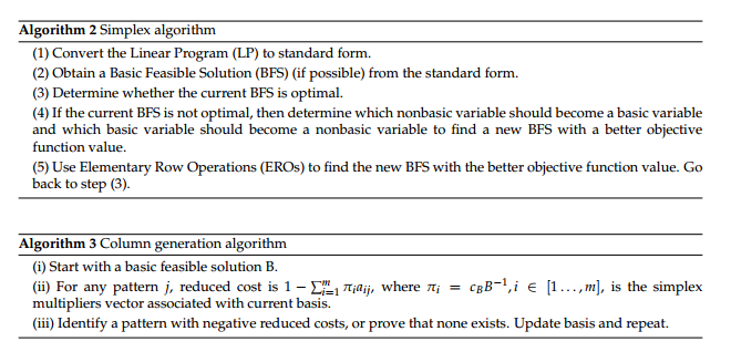
Further explanation can be obtain in [24]. Now that we have defined the two algorithms, we proceed to the experiments as given in the next section.

3.Result

Our experimental results for the problems are given here. We use the branch and bound algorithm to solve TSP and column generation technique to solve CVRP.

Experiment 1: branch-and-cut (BAC) with TSP

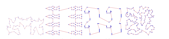
This section presents the performance tests of branch and cut algorithm on Euclidean instances of TSPLIB library. The tests were performed on a computer processor intel(R) core (TM) i5-2450m cpu 2.60GHZ @ 2.60GHT and 8GB of Ram. The adaptation of the proposed algorithm is coded into a python programming language version \(3.6 \) . Result obtained by applying the exact method in solving the symmetric TSP problem is summarized in the tables below.

Table 1. Branch-and-cut result.

Instances	Number of Instance	Best Known Solution	BAC Method	Time(sec)	Error(\%)
Wi29	29	27603	27603	0.10	0.0
DJ38	38	6656	6656	0.12	0.0
Berlin52	52	7542	7542	0.15	0.0
pr76	76	21282	21282	0.66	0.0
KroA100	100	108159	108159	0.62	0.0
pr136	136	96772	96772	0.44	0.0
pr144	144	58537	58537	1.63	0.0
ch150	150	6528	6528	7.44	0.0
qa194	194	9352	9352	1.83	0.0
KroA200	200	29437	29437	1.61	0.0

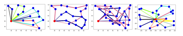
The Table 1 shows the results obtained when Exact method was applied on TSP instance. The method give optimality. The optimal tour for these instances are shown in Figures (1),(2) and (3).

Experiment 2: column generation applied on CVRP

The Column Generation (CG) method is an exact method for solving the CVRP and the VRP in general, this technique has been explicitly explained and gives an optimal solution to a problem.

The Table 2 gives the summary of the comparison of this technique's primal and dual problem, since CG work on dual solution of the relaxed master problem, their optimal gap in percentage. The Table 2 consists of seven columns: Instances (contains the instances written as \(P-n16-k8\) which means the data consists of \(16\) nodes with \(8\) fleets of vehicles), Cities (locations to be visited), Best value (from literature), Relaxed Master Problem (RMP), Column Generation (based on dual values), column generation computational time and optimality gap. From the Table , the optimal gap for all the instances considered gives 0.00%. From the instances we consider in this research, only coordinates and demands for each nodes are given, CG compute the distance between two coordinates; \((x_{1}, y_{1})\), \((x_{2}, y_{2})\), using the Euclidean formula:

Table 2. Column generation result.

Instances	Cities	Best value	RMP (primal)	result (C(S))	CG time	gap
P-n16-k8	16	450	450	450.00	14.72	0.00%
P-n20-k2	20	220	220	220.00	38.64	0.00%
P-n22-k2	22	216	216	216.00	44.31	0.00%
P-n22-k8	22	603	603	603.00	19.66	0.00%
P-n40-k5	39	458	458	458.00	32.22	0.00%
P-n50-k10	49	696	696	696.00	38.42	0.00%
P-n101-k4	100	681	681	681.00	39.16	0.00%

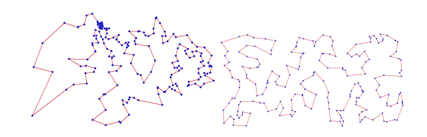
To obtain the optimality gap between the two results, we use the formula in (15). These results were obtained using gurobi solver in python [23]. The optimal tours for the first four instances are given in Figure (4)below.

So far we considered only two variants of the vehicle routing problem which are: travelling salesman problem and capacitated vehicle routing problem. For the travelling salesman problem, we used branch and cut algorithm to solve the problem and applied it on some instances. We considered the following TSPLIB instance; Wi29, DJ38, Berlin52, Pr76, KroA100, pr136, pr144, ch150, qa19 and KroA200. Since technique produced an optimal solution, which ascertain the fact that exacts methods give optimal solutions. The results are shown in the Table (1). For the capacitated vehicle routing problem, we used column generation technique to solve this mathematical model and applied it on Augerat et al. (E) data. These technique produced optimal solutions as well. The results are given in the Table (2).

4.Conclusion

In this research work, we solved Travelling Salesman Problem and Capacitated Vehicle Routing Problem using branch-and-cut and column generation algorithms, respectively. These techniques: branch-and-bound and column generation produced optimal solutions for travelling salesman problem and capacitated vehicle routing problem respectively. Other variants of Vehicle Routing Problem can also be solved using other exact algorithms.

In future, we can use machine learning techniques such as Neural combinatorial optimization approach to solve the Vehicle Routing Problems.

acknowledgments

The authors would like to express their thanks to the referee for his useful remarks.

Authorcontributions

All authors contributed equally to the writing of this paper. All authors read and approved the final manuscript.

Conflictofinterests

The authors declare no conflict of interest.

References

1. Ibrahim, A. A., Lo, N., Abdulaziz, R. O., & Ishaya, J. A. (2019). Capacitated vehicle routing problem. International Journal of Research-Granthaalayah, 7(3), 310-327. [Google Scholor]
2. Toth, P., & Vigo, D. (2002). An overview of vehicle routing problems. In The vehicle routing problem (pp. 1-26). Society for Industrial and Applied Mathematics. [Google Scholor]
3. Golden, B. L., Raghavan, S., & Wasil, E. A. (Eds.). (2008). The vehicle routing problem: latest advances and new challenges (Vol. 43). Springer Science & Business Media. [Google Scholor]
4. Laporte, G. (1992). The vehicle routing problem: An overview of exact and approximate algorithms. European journal of operational research, 59(3), 345-358. [Google Scholor]
5. Semet, F., Toth, P., & Vigo, D. (2014). Chapter 2: Classical exact algorithms for the capacitated vehicle routing problem. In Vehicle Routing: Problems, Methods, and Applications, Second Edition (pp. 37-57). Society for Industrial and Applied Mathematics. [Google Scholor]
6. Beltrami, E. J., & Bodin, L. D. (1974). Networks and vehicle routing for municipal waste collection. Networks, 4(1), 65-94. [Google Scholor]
7. Kallehauge, B., Larsen, J., Madsen, O. B., & Solomon, M. M. (2005). Vehicle routing problem with time windows. In Column generation (pp. 67-98). Springer, Boston, MA. [Google Scholor]
8. Cappanera, P., Gouveia, L., & Scutellà, M. G. (2011, June). The skill vehicle routing problem. In International Conference on Network Optimization (pp. 354-364). Springer, Berlin, Heidelberg. [Google Scholor]
9. Chauhan, C., Gupta, R., & Pathak, K. (2012). Survey of methods of solving tsp along with its implementation using dynamic programming approach. International journal of computer applications, 52(4). [Google Scholor]
10. Edwards, C., & Spurgeon, S. (1998). Sliding mode control: theory and applications. Crc Press. [Google Scholor]
11. Dantzig, G. B., & Ramser, J. H. (1959). The truck dispatching problem. Management science, 6(1), 80-91. [Google Scholor]
12. Geldenhuys, C. E. (1998). An implementation of a branch-and-cut algorithm for the travelling salesman problem (Doctoral dissertation, University of Johannesburg). [Google Scholor]
13. Padberg, M., & Rinaldi, G. (1991). A branch-and-cut algorithm for the resolution of large-scale symmetric traveling salesman problems. SIAM review, 33(1), 60-100.[Google Scholor]
14. Desrochers, M., Desrosiers, J., & Solomon, M. (1992). A new optimization algorithm for the vehicle routing problem with time windows. Operations research, 40(2), 342-354. [Google Scholor]
15. Kohl, N., Desrosiers, J., Madsen, O. B., Solomon, M. M., & Soumis, F. (1999). 2-path cuts for the vehicle routing problem with time windows. Transportation Science, 33(1), 101-116. [Google Scholor]
16. Choi, E., & Tcha, D. W. (2007). A column generation approach to the heterogeneous fleet vehicle routing problem. Computers & Operations Research, 34(7), 2080-2095.[Google Scholor]
17. Gendreau, M., Guertin, F., Potvin, J. Y., & Saguin, R. (2006). Neighborhood search heuristics for a dynamic vehicle dispatching problem with pick-ups and deliveries. Transportation Research Part C: Emerging Technologies, 14(3), 157-174. [Google Scholor]
18. Hvattum, L. M., Lkketangen, A., & Laporte, G. (2006). Solving a dynamic and stochastic vehicle routing problem with a sample scenario hedging heuristic. Transportation Science, 40(4), 421-438.[Google Scholor]
19. Brotcorne, L., Laporte, G., & Semet, F. (2003). Ambulance location and relocation models. European journal of operational research, 147(3), 451-463. [Google Scholor]
20. Claassen, G. D. H., & Hendriks, T. H. (2007). An application of special ordered sets to a periodic milk collection problem. European Journal of Operational Research, 180(2), 754-769. [Google Scholor]
21. Curtin, K. M., Voicu, G., Rice, M. T., & Stefanidis, A. (2014). A comparative analysis of traveling salesman solutions from geographic information systems. Transactions in GIS, 18(2), 286-301. [Google Scholor]
22. van Lent, G. P. T. (2018). Using column generation for the time dependent vehicle routing problem with soft time windows and stochastic travel times (Master's thesis). [Google Scholor]
23. Inc. gurobi optimization. gurobi optimizer reference manual, 2019, url, http://www.gurobi. com, 2019. [Google Scholor]
24. Winston, W. L., & Goldberg, J. B. (2004). Operations research: applications and algorithms (Vol. 3). Belmont: Thomson Brooks/Cole. [Google Scholor]