
Humanity has been severely affected by many epidemics throughout history, and we can say that this situation continues in today’s world, which is still developing in every sense. The area of mathematical epidemiology, in which epidemics are examined by mathematical modeling and analysis of the formed model, appeals to compartmental modeling to examine the dynamics of the epidemic. By using compartmental models, forecasts can be made regarding the course of diseases and behavioral dynamics, [1,2,3].
It is often preferable to speak with integer parameter values for transmission ratios between classes when working with compartmental models, but this situation may not always accurately reflect reality. It is generally thought to replace the integer value corresponding to a parameter with its interval value to express the observation process’s variability or uncertainty. In this context, we consider replacing integer-valued parameters and functions with interval-valued ones to perform a more robust evaluation and analysis related to disease spreading. So, in this study, it is assumed that the coefficient rates remain within known intervals, even though they change over time.
In mathematical epidemiology, some models, including the discrete-time difference equations and using interval-valued parameters have been proposed for state estimations related to the course of diseases (see, e.g., [4,5,6,7,8,9]). In addition, the authors [10,11,12] have dealt with interval observers for uncertain dynamical systems. However, the literature lacks the studies in which stabilities of continuous-time dynamical systems with interval-valued parameters and functions are examined. With this study, it is aimed to present a different interpretation of interval-valued approach styles to the field of mathematical epidemiology.
This study has proposed a new model involving the effect of isolation and the interval-valued parameters and functions for analyzing the course of the spread of epidemic disease in a population. The paper focuses on the global stability of a continuous-time \(SEIR\) epidemic model under isolation effect. The model built in the study is designed by an approach with interval coefficients to observe the possible results of the behavioral movement of the epidemic. This approach is based on a coherent extension of traditional integer coefficients’ compartmental modeling technique. It is assumed that parameters and functions from each compartment stage in the model remains within a specific bounded interval. To apply the aimed interval approach to the epidemic model, it has been presented the transmission dynamics in the compartmental system explaining the outbreak, in two parts as the systems (15) and (16), using the lower and upper endpoints of the interval-valued parameters defining them. To observe the changes in population density in each compartment of the system at any time \(t\), it would be more appropriate to analyze these two subsystems separately. After calculating the interval that will occur for the value \(\mathcal{R}_{0}\), known as the number of secondary infections, the qualitative and stability analysis results for the subsystems, which are evaluated separately with the lower and upper endpoints of the parameters and functions, have been given. After the subsystems’ local and global asymptotic stability has been shown, these results have been combined with functional analysis methods. So, it has been concluded that the stability of the proposed epidemic model.
This study has established a new \(SEIR\) model to examine the course of an epidemic with interval-valued parameters and functions under isolation effect. To use this interval perspective, it may be helpful to get acquainted with the theory on which it is based, quasilinear spaces (see, [13]). To this journey from quasilinear structures to population dynamics, we will begin by defining quasilinear space, in which the set \(\Omega _{C}\left( \mathbb{R}\right) \), that interval coefficients are taken, belongs to it. The basic definition related to the quasilinear spaces given by Aseev has been presented as follows.
Definition 1. A set \(X\) is called quasilinear space if a partial order relation “\(\preceq \)” , an algebraic sum operation and an operation of multiplication by real numbers are defined in it in such a way that the following conditions hold for any elements \(x,y,z,v\in X\) and any \(\alpha ,\beta \in \mathbb{R} \):
Also, it will be assumed throughout the text that \(-x=(-1)\cdot x\).
As a set that does not have a linear space structure and carries a quasilinear space structure, one of the most important examples is the set of all nonempty, compact and convex subsets of real numbers with the inclusion relation “\(\subseteq \)” \(.\) This set is denoted by \(\Omega _{C}\left( \mathbb{R}\right) \) and the algebraic sum operation and multiplication operation by a real number \(\lambda \) on \( \Omega _{C}\left( \mathbb{R}\right) \) are defined as
\begin{equation*} A+B=\left\{ a+b:a\in A,\text{ }b\in B\right\} \end{equation*} and \begin{equation*} \lambda \cdot A=\left\{ \lambda a:a\in A\right\} . \end{equation*} This set consisting of intervals in \(\mathbb{R}\) forms the basis of interval analysis. Interval analysis has been used in many areas, including practical application areas such as behavioral ecology, economics, chemical, and structural engineering, beam physics, signal processing, robotics, constraint satisfaction, control circuitry design, etc. Interval methods used commonly in these areas can give distinctive bounds for various problems such as global optimization, parameter estimation, control theory, motion planning, set estimation, and stability analysis. The reader can benefit from [14] and [15] and the references therein to provide an introduction to the theory and methods of interval analysis.On the other hand, many details about the theory of quasilinear spaces have been investigated and exemplified on the set \(\Omega _{C}\left( \mathbb{R} \right) \) at the first stage. Çakan and Yi lmaz [16,17,18,19] ; Bozkurt and Yi lmaz [20,21,22,23,24,25,26,27,28]; Dehghanizade and Modarres [29] have strived to extend the theory of quasilinear spaces with various perspectives utilizing the interval-valued functions, too. The reader can review the authors’ these studies and references therein, for details concerning basic definitions and notions about the theory of quasilinear spaces.
While modeling on disease dynamics, we will focus on the set \(\Omega _{C}\left( \mathbb{R}\right) \), from which we choose the coefficients that determine the dynamics of the model. Therefore, we will give a general summary of some basic concepts related to the theory of intervals, which are the elements of \(\Omega _{C}\left( \mathbb{R}\right) \). The following passages are taken from the author’s study in [30] and references cited therein for related parts.
For \(\left[ \underline{A},\overline{A}\right] \), \(\left[ \underline{B}, \overline{B}\right] \in \Omega _{C}\left( \mathbb{R}\right) \) and \(\lambda \in \mathbb{R},\) the usual interval operations, i.e. Minkowski addition and scalar multiplication are defined as
\begin{equation*} \left[ \underline{A},\overline{A}\right] +\left[ \underline{B},\overline{B} \right] =\left[ \underline{A}+\underline{B},\overline{A}+\overline{B}\right] \end{equation*} and \begin{equation*} \lambda \cdot \left[ \underline{A},\overline{A}\right] =\left\{ \begin{array}{cc} \left[ \lambda \underline{A},\lambda \overline{A}\right] , & \lambda >0 \\ \left\{ 0\right\} , & \lambda =0 \\ \left[ \lambda \overline{A},\lambda \underline{A}\right] , & \lambda < 0 \end{array} \right. , \end{equation*} respectively. Also \((-1)\cdot \left[ \underline{A},\overline{A}\right] =- \left[ \underline{A},\overline{A}\right] =\left[ -\overline{A},-\underline{A} \right] .\)For the metric structure given by the Hausdorff-Pompeiu distance on \(\Omega _{C}\left( \mathbb{R}\right) \) see [30].
We denote the width of an interval \(A=\left[ \underline{A},\overline{A} \right] \) by \(w(A)=\overline{A}-\underline{A}.\)
Also we say that an interval valued function \(F:\left[ a,b\right] \rightarrow \Omega _{C}\left( \mathbb{R}\right) \) is \(w-\)increasing (\(w-\) decreasing) on \(\left[ a,b\right] ,\) if the real function \(w_{F}:\left[ a,b \right] \rightarrow \mathbb{R}^{+}\) defined by \(w_{F}(t)=w\left( F(t)\right) \) is increasing (decreasing) on \(\left[ a,b\right] \). We say that \(F\) is \(w-\) monotone on \(\left[ a,b\right] \) if \(w_{F}\) is \(w-\)increasing or \(w-\) decreasing, [31].
The generalized Hukuhara difference (or gH -difference) of two intervals \( \left[ \underline{A},\overline{A}\right] \), \(\left[ \underline{B},\overline{B }\right] \in \Omega _{C}\left( \mathbb{R}\right) \) is defined as follows
\begin{equation*} \left[ \underline{A},\overline{A}\right] \ominus _{g}\left[ \underline{B}, \overline{B}\right] =\left[ \min \left\{ \underline{A}-\underline{B}, \overline{A}-\overline{B}\right\} ,\max \left\{ \underline{A}-\underline{B}, \overline{A}-\overline{B}\right\} \right] . \end{equation*}Definition 2. [31] Let \(F:[a,b]\rightarrow \Omega _{C}\left( \mathbb{R}\right) \) be an interval valued function, \(t_{0}\in \lbrack a,b]\) and define \( F^{\prime }(t_{0})\in \Omega _{C}\left( \mathbb{R}\right) \) (if it exists) as \begin{equation*} F^{\prime }(t_{0})=\underset{h\rightarrow 0}{\lim }\frac{F(t_{0}+h)\ominus _{g}F(t_{0})}{h}. \end{equation*} Then it is said that \(F^{\prime }(t_{0})\) is generalized Hukuhara derivative (gH-derivative, for short) of \(F\) at \(t_{0}\). Also we say that \(F\) is generalized Hukuhara differentiable (gH-differentiable, for short) on \([a,b]\) if \(F^{\prime }(t)\in \Omega _{C}\left( \mathbb{R}\right) \) exists at each point \(t\in \lbrack a,b]\). Then the interval valued function \(F^{\prime }:[a,b]\rightarrow \) \(\Omega _{C}\left( \mathbb{R}\right) \) is called gH-derivative of \(F\) on \([a,b].\)
Proposition 1. [31] Let \(F:[a,b]\rightarrow \Omega _{C}\left( \mathbb{ R}\right) \) be an interval valued function such that \(F(t)=[\underline{F(t)}, \overline{F(t)}]\) for \(t\in \lbrack a,b].\) If the real-valued functions \( \underline{F}\) and \(\overline{F}\) are differentiable at \(t\in \lbrack a,b]\) then \(F\) is gH-differentiable at \(t\in \lbrack a,b]\) and
It is known that \(C\left[ a,b\right] \) which is the family of all real valued and continuous functions defined on interval \(\left[ a,b\right] \) is a complete metric space with the standard metric
\begin{equation*} h\left( f,g\right) =\max \left\{ \left\vert f(t)-g(t)\right\vert :t\in \left[ a,b\right] \right\} . \end{equation*} Let \(C\left( \left[ a,b\right] ,\Omega _{C}\left( \mathbb{R}\right) \right) \) denote the set of all continuous interval valued functions defined on \(\left[ a,b\right] \). One can see the metric structure on \(C\left( \left[ a,b\right] ,\Omega _{C}\left( \mathbb{R}\right) \right) \) in [30].The Lebesgue integral for interval valued functions is a special case of the Lebesgue integral for set-valued mappings, [32].
Let \(F:[a,b]\rightarrow \Omega _{C}\left( \mathbb{R}\right) \) be an interval valued function such that \(F(t)=[\underline{F(t)},\overline{F(t)}]\) and \( \underline{F},\) \(\overline{F}\) are measurable and Lebesgue integrable on \( [a,b]\). Then it said that \(F\) is Lebesgue integrable on \([a,b]\) and
\begin{equation*} \int\limits_{a}^{b}F(t)dt=\left[ \int\limits_{a}^{b}\underline{F(t)} dt,\int\limits_{a}^{b}\overline{F(t)}dt\right] . \end{equation*}Unlike the classical aspect of compartmental models, in this paper we assume that \(X\left( t\right) \) describes the interval of the number of individuals in compartment \(X\) at time \(t.\) That is, \(X\left( t\right) =\left[ \underline{X}\left( t\right) ,\overline{X}\left( t\right) \right] \) and the number of individuals in \(X\) takes value into this interval.
The model formed as lower and upper system under the isolation effect is as follows:
Let \(N\) show the total population consisting the compartments \(S,\) \(E,\) \(I,\) \(R\) which represent the compartments consisting individuals of S usceptible against the disease, Exposed to the disease, I nfectious and Removed from the disease, respectively. Alongside this, the \(N\left( t\right) ,\) \(S\left( t\right) ,\) \(E\left( t\right) ,\) \( I\left( t\right) ,\) \(R\left( t\right) \) describe the numbers of individuals in the relevant compartments at time \(t\). These variables are undoubtedly non-negative and it is no wonder that
\begin{equation*} \underline{S}\left( t\right) =N\left( t\right) -\overline{E}\left( t\right) – \overline{I}\left( t\right) -\overline{R}\left( t\right) \end{equation*} and \begin{equation*} \overline{S}\left( t\right) =N\left( t\right) -\underline{E}\left( t\right) – \underline{I}\left( t\right) -\underline{R}\left( t\right) \end{equation*} for all \(t\geq 0.\)As with all classic mathematical epidemic models, it is assumed that all newborn members are directly included in the susceptible compartment. All parameters reflecting transitions between the compartments in the model are non-negative constants and are given in the Table 1 along with their meanings.
| Parameter | Description |
|---|---|
| \(\underline{\Lambda }\) \(\left( \overline{\Lambda }\right) \) | lower (upper)bound for birth rate |
| \(\underline{\omega }\)\(\left( \overline{\omega }\right) \) | lower (upper)bound for isolation rate |
| \(\underline{\beta }\) \(\left( \overline{\beta }\right) \) | lower (upper)bound for effective contact rate between infectious and susceptible |
| \(\underline{\mu }\) \(\left( \overline{\mu }\right) \) | lower (upper) boundfor natural death rate of all compartments |
| \(\underline{\delta }\)\(\left( \overline{\delta }\right) \) | lower (upper)bound for progression rate of exposed individuals into infectious compartment |
| \(\underline{p}\) \(\left( \overline{p}\right) \) | lower (upper) bound for thetransition rate from exposed class to the compartment $R$ |
| \(\underline{q\text{ }}\left( \overline{q}\right) \) | lower (upper) bound forthe transition rate from infectious class to the compartment $R$ |
| \(\underline{d}\) \(\left( \overline{d}\right) \) | lower (upper) bound fordeath rate derived from disease causing to outbreak |
The parameter \(\left[ \underline{\omega },\overline{\omega }\right] \), which is included by the interval \(\left[ 0,1\right] \), represents the level of isolation. As might be expected, the case \(\underline{\omega }=\overline{ \omega }=0\) means that isolation has not applied, the case \(\underline{ \omega }=\overline{\omega }=1\) says that isolation has been strictly and fully implemented.
Further, \(\tau \) is time delay corresponding to the latent period of the disease. The numbers of exposed to disease and still surviving individuals at the time \(t\) are mathematically explained shaped \(\underline{\beta } \underline{S}\left( t-\tau \right) \underline{I}\left( t-\tau \right) e^{- \underline{\mu }\tau }\) for the model (15) and \(\overline{ \beta }\overline{S}\left( t-\tau \right) \overline{I}\left( t-\tau \right) e^{-\overline{\mu }\tau }\) for the model (16), respectively.
To consider the models on these sets will be enough to examine mathematically and epidemiologically.
The proof for positive invariance has been neglected for this study to avoid similar steps. However, one can examine the references presented in [3,33] for details of a similar proof.
The regions \(\underline{\Psi }\) and \(\overline{\Psi }\) attract all intervals consisting of solutions of the systems (15) and (16), respectively. These restricted regions determine the bounds which will be enough to investigate the behavioral dynamics regarding the stability of the model.
Since the variables \(\underline{E}\left( t\right) ,\underline{R}\left( t\right) \) and \(\overline{E}\left( t\right) ,\) \(\overline{R}\left( t\right) \) do not appear in other remaining equations of system (15) and (16), respectively, we can only consider the subsystems consisting of the first and third equations in these systems.
Thus the reduced model, which is taken into account the effect of isolation rate is as follows with a time delay representing the latent period:
We will calculate the primary reproduction number defined as the epidemic threshold of a particular infection for our model. A suggested approach to determining the value \(\mathcal{R}_{0}\), next-generation matrix method, is detailed in [34] and [35]. Generations in epidemic models are the waves of secondary infection that flow from each previous infection. In this way, the course of the disease towards persistence or disappearance can be predicted by this critical threshold.
In this study, unlike the classical approaches, we consider the threshold \( \mathcal{R}_{0}\) as a value that can change between the boundaries of an interval, instead of expressing as an integer. So, we represent this value by \(\mathcal{R}_{0}=\left[ \min \left\{ \underline{\mathcal{R}_{0}}, \overline{\mathcal{R}_{0}}\right\} ,\max \left\{ \underline{\mathcal{R}_{0}}, \overline{\mathcal{R}_{0}}\right\} \right] \). In this way, in cases where there is a lack of information in the parameter values, the number of secondary infections are taken as the interval formed by the formulas that come with the lower and upper endpoints of the intervals in which the parameters are limited. Thus the uncertainties will be limited within a particular interval and the margin of error will be reduced.
To compute \(\underline{\mathcal{R}_{0}}\), the variables in subsystem (17) are ordered first according to the infectious states \(\left( \mathcal{F}\left( \underline{X}\right) \right) \) and then according to the other states \(\left( \mathcal{V}\left( \underline{X}\right) \right) \) as follows.
Let be defined as \(\underline{X}=(\underline{I},\underline{S})^{T}\) and the reduced subsystem (17) be expressed as
Similarly we get
On the other hand, for the endemic equilibrium point which will be represent as \(\underline{P_{\ast }}=\left( \underline{S^{\ast }},\underline{I^{\ast }} \right) \) of system (17) we get the solutions
\begin{equation*} \underline{S^{\ast }}=\frac{\underline{q}+\underline{\mu }+\underline{d}}{ \underline{\delta }\left( 1-\underline{\omega }\right) \underline{\beta }e^{- \underline{\mu }\tau }}, \end{equation*} and \begin{equation*} \underline{I^{\ast }}=\frac{\underline{\Lambda }\underline{\delta }\left( 1- \underline{\omega }\right) \underline{\beta }e^{-\underline{\mu }\tau }- \underline{\mu }\left( \underline{q}+\underline{\mu }+\underline{d}\right) }{ \left( \underline{q}+\underline{\mu }+\underline{d}\right) \left( 1- \underline{\omega }\right) \underline{\beta }} \end{equation*} from the algebraic equationsTheorem 1. If \(\underline{\mathcal{R}_{0}}< 1\) then the disease-free equilibrium point \( \underline{P_{0}}\) is locally asymptotically stable in \(\underline{\Psi }\).
Proof. For subsystem (17), the Jacobian matrix at disease-free equilibrium \(\underline{P_{0}}\) is \begin{equation*} \underline{J}\left( \underline{P_{0}}\right) = \begin{bmatrix} -\left( 1-\underline{\omega }\right) \underline{\beta }\underline{I_{0}}- \underline{\mu } & & -\left( 1-\underline{\omega }\right) \underline{\beta } \underline{S_{0}} \\ & & \\ \underline{\delta }\left( 1-\underline{\omega }\right) \underline{\beta } \underline{I_{0}}e^{-\underline{\mu }\tau } & & \underline{\delta }\left( 1- \underline{\omega }\right) \underline{\beta }\underline{S_{0}}e^{-\underline{ \mu }\tau }-\left( \underline{q}+\underline{\mu }+\underline{d}\right) \end{bmatrix} \end{equation*} and the characteristic equation which is correspond to the matrix formed by considered \(\underline{S_{0}}=\underline{\Lambda }/\underline{\mu }\) and \( \underline{I_{0}}=\underline{0}\) is
Theorem 2. If \(\overline{\mathcal{R}_{0}}< 1\) then the disease-free equilibrium point \( \overline{P_{0}}\) is locally asymptotically stable in \(\overline{\Psi }\).
Proof. By following again similar steps to proof of the previous theorem, the roots of the characteristic equation
Theorem 3. If \(\underline{\mathcal{R}_{0}}>1,\) the endemic equilibrium point \( \underline{P_{\ast }}\) is locally asymptotically stable in \(\underline{\Psi } \).
Proof. For system (17), the Jacobian matrix at the endemic equilibrium \(\underline{P_{\ast }}=\left( \underline{S^{\ast }},\underline{ I^{\ast }}\right) \) is \begin{equation*} \underline{J}\left( \underline{P_{\ast }}\right) = \begin{bmatrix} -\left( 1-\underline{\omega }\right) \underline{\beta }\underline{I^{\ast }}- \underline{\mu } & & -\left( 1-\underline{\omega }\right) \underline{\beta } \underline{S^{\ast }} \\ & & \\ \underline{\delta }\left( 1-\underline{\omega }\right) \underline{\beta } \underline{I^{\ast }}e^{-\underline{\mu }\tau } & & \underline{\delta } \left( 1-\underline{\omega }\right) \underline{\beta }\underline{S^{\ast }} e^{-\underline{\mu }\tau }-\left( \underline{q}+\underline{\mu }+\underline{d }\right) \end{bmatrix} . \end{equation*} Taking into account \begin{equation*} \underline{S^{\ast }}=\frac{\underline{\Lambda }}{\underline{\mu }\underline{ \mathcal{R}_{0}}}\text{ and } \underline{I^{\ast }}=\frac{ \underline{\mu }}{\left( 1-\underline{\omega }\right) \underline{\beta }} \left( \underline{\mathcal{R}_{0}}-1\right) , \end{equation*} the matrix \(\underline{J}\left( \underline{P_{\ast }}\right) \) is obtained as \begin{equation*} \underline{J}\left( \underline{P_{\ast }}\right) = \begin{bmatrix} \underline{\mu }\underline{\mathcal{R}_{0}} & & -\frac{\underline{\Lambda } \left( 1-\underline{\omega }\right) \underline{\beta }}{\underline{\mu } \underline{\mathcal{R}_{0}}} \\ & & \\ \underline{\delta }\underline{\mu }e^{-\underline{\mu }\tau }\left( \underline{\mathcal{R}_{0}}-1\right) & & 0 \end{bmatrix} . \end{equation*} Then \begin{equation*} tr\left( \underline{J}\left( \underline{P_{\ast }}\right) \right) =- \underline{\mu }\underline{\mathcal{R}_{0}}0. \end{equation*} Thus both eigenvalues of \(\underline{J}\left( \underline{P_{\ast }}\right) \) have negative real parts for \(\underline{\mathcal{R}_{0}}>1\) and so the endemic equilibrium \(\underline{P_{\ast }}\) is locally asymptotically stable in the set \(\underline{\Psi }.\)
Theorem 4. If \(\overline{\mathcal{R}_{0}}>1,\) the endemic equilibrium point \(\overline{ P_{\ast }}\) is locally asymptotically stable in \(\overline{\Psi }\).
Proof. Proof can be made similarly to previous proof.
Theorem 5. If \(\underline{\mathcal{R}_{0}}< 1\) then the disease-free equilibrium point \( \underline{P_{0}}\) is globally asymptotically stable in \(\underline{\Psi }\).
Proof. Let us consider a nonnegative function \(L_{low}\) specifically defined as \begin{equation*} L_{low}\left( t\right) =\underline{I}\left( t\right) +\underline{\delta } \left( 1-\underline{\omega }\right) \underline{\beta }e^{-\underline{\mu } \tau }\int\limits_{t-\tau }^{t}\underline{S}\left( x\right) \underline{I} \left( x\right) dx. \end{equation*} It is clear that \(L_{low}=0\) at \(\underline{P_{0}}=\left( \underline{S_{0}}, \underline{I_{0}}\right) .\) Also from the time derivative of function \( L_{low}\), it is obtained that \begin{eqnarray*} \frac{dL_{low}}{dt} &=&\frac{d\underline{I}\left( t\right) }{dt}+\underline{ \delta }\left( 1-\underline{\omega }\right) \underline{\beta }e^{-\underline{ \mu }\tau }\left[ \underline{S}\left( t\right) \underline{I}\left( t\right) – \underline{S}\left( t-\tau \right) \underline{I}\left( t-\tau \right) \right] \\ &=&\underline{\delta }\left( 1-\underline{\omega }\right) \underline{\beta } \underline{S}\left( t-\tau \right) \underline{I}\left( t-\tau \right) e^{- \underline{\mu }\tau }-\left( \underline{q}+\underline{\mu }+\underline{d} \right) \underline{I}\left( t\right) \\ &&+\underline{\delta }\left( 1-\underline{\omega }\right) \underline{\beta } \underline{S}\left( t\right) \underline{I}\left( t\right) e^{-\underline{\mu }\tau }-\underline{\delta }\left( 1-\underline{\omega }\right) \underline{ \beta }\underline{S}\left( t-\tau \right) \underline{I}\left( t-\tau \right) e^{-\underline{\mu }\tau } \\ &=&\underline{I}\left( t\right) \left( \underline{\delta }\left( 1- \underline{\omega }\right) \underline{\beta }\underline{S}\left( t\right) e^{-\underline{\mu }\tau }-\left( \underline{q}+\underline{\mu }+\underline{d }\right) \right) \\ &\leq &\left( \underline{q}+\underline{\mu }+\underline{d}\right) \underline{ I}\left( t\right) \left( \frac{\underline{\delta }\left( 1-\underline{\omega }\right) \underline{\beta }\underline{\Lambda }e^{-\underline{\mu }\tau }}{ \underline{\mu }\left( \underline{q}+\underline{\mu }+\underline{d}\right) } -1\right) \\ &=&\left( \underline{q}+\underline{\mu }+\underline{d}\right) \underline{I} \left( t\right) \left( \underline{\mathcal{R}_{0}}-1\right) . \end{eqnarray*} While \(\underline{\mathcal{R}_{0}}< 1,\) \(dL_{low}/dt\leq 0\) and \( dL_{low}/dt=0\) only at \(\underline{P_{0}}\). So \(L_{low}\) satisfies the conditions being the Lyapunov function. With LaSalle's Invariance Principle, we say that solutions of (17) has limit in the largest invariant subset of \begin{equation*} \left\{ \left( \underline{S}\left( t\right) ,\underline{I}\left( t\right) \right) :\left( \underline{S}\left( t\right) ,\underline{I}\left( t\right) \right) \text{ is a solution of }\frac{dL_{low}}{dt}=0\right\} . \end{equation*} Also we immediately note that this subset consists only \(\underline{P_{0}}\). This means that all solutions of (17) tend to \( \underline{P_{0}}\) if \(\underline{\mathcal{R}_{0}}< 1\). Therefore \(\underline{ P_{0}}\) is globally asymptotically stable in \(\underline{\Psi }.\)
Theorem 6. The disease-free equilibrium point \(\overline{P_{0}}\) is globally asymptotically stable in \(\overline{\Psi }\) for \(\overline{\mathcal{R}_{0}} >1 \).
Proof. The proof bases on constructing of a Lyapunov function (similarly \(L_{low}\)) defined with the help of the upper endpoints of the intervals formed by the relevant parameters and functions and
Theorem 7. The endemic equilibrium point \(\underline{P_{\ast }}\) is globally asymptotically stable in \(\underline{\Psi }\) for \(\underline{\mathcal{R}_{0}} >1\).
Proof. Firstly, let us consider the function \(\varphi :\left( 0,\infty \right) \rightarrow \left[ 0,\infty \right) \) defined as \(\varphi \left( z\right) =z-1-\ln z\) for \(z>0.\) For this function it is clear that \(\varphi \left( z\right) \geq 0\) and \(\varphi \) reaches \(0\) which is its global minimum value at \(1\). Now, let us consider the function \(W_{low}\) constructed by means of \(\varphi \), defined as \begin{equation*} W_{low}(t)=W_{low1}(t)+W_{low2}(t)+W_{low3}(t) \end{equation*} such that \begin{eqnarray*} W_{low1}(t) &=&\underline{S^{\ast }}\text{ }\varphi \left( \frac{\underline{S }\left( t-\tau \right) }{\underline{S^{\ast }}}\right) , \\ W_{low2}(t) &=&\frac{e^{\underline{\mu }\tau }}{\underline{\delta }} \underline{I^{\ast }}\text{ }\varphi \left( \frac{\underline{I}\left( t\right) }{\underline{I^{\ast }}}\right) , \\ W_{low3}(t) &=&\underline{\beta }\underline{S^{\ast }}\underline{I^{\ast }} \int\limits_{t-\tau }^{t}\varphi \left( \frac{\underline{I}\left( x\right) }{ \underline{I^{\ast }}}\right) dx. \end{eqnarray*} It is clear that \(W_{low}=0\) only at \(\left( \underline{S^{\ast }}, \underline{I^{\ast }}\right) .\)
To check whether the conditions required for \(W_{low}\) to be a Lyapunov function is satisfied or not, we need to examine the time derivative of this function. In order to ease the tracking of mathematical operations, we will calculate the derivatives of \(W_{low1},\) \(W_{low2}\) and \(W_{low3}\) separately and combine them in the last part.
Firstly, we obtain time derivatives of functions \(W_{low1}\) and \(W_{low2}\) as
On the other hand, \(dW_{low}/dt=0\) if and only if
\begin{equation*} \left( 2-\frac{\underline{S}\left( t-\tau \right) }{\underline{S^{\ast }}}- \frac{\underline{S^{\ast }}}{\underline{S}\left( t-\tau \right) }\right) =0, \end{equation*} \begin{equation*} \left( 1-\frac{\underline{S^{\ast }}}{\underline{S}\left( t-\tau \right) } +\ln \frac{\underline{S^{\ast }}}{\underline{S}\left( t-\tau \right) } \right) =0 \end{equation*} and \begin{equation*} \left( 1-\frac{\underline{S}\left( t-\tau \right) \underline{I}\left( t-\tau \right) }{\underline{I}\left( t\right) \underline{S^{\ast }}}+\ln \frac{ \underline{S}\left( t-\tau \right) \underline{I}\left( t-\tau \right) }{ \underline{I}\left( t\right) \underline{S^{\ast }}}\right) =0. \end{equation*} So, it is obtained that \(\underline{S}\left( t-\tau \right) =\underline{ S^{\ast }}\) and \(\underline{I}\left( t-\tau \right) =\underline{I}\left( t\right) .\) Now anymore the largest invariant subset can be searched within the set \begin{equation*} \left\{ \left( \underline{S}\left( t\right) ,\underline{I}\left( t\right) \right) :\underline{S}\left( t\right) =\underline{S^{\ast }}\text{ and } \underline{I}\left( t-\tau \right) =\underline{I}\left( t\right) \right\} . \end{equation*} Since \(\underline{S}\left( t\right) =\underline{S^{\ast }},\) we have \begin{eqnarray*} \frac{d\underline{S}}{dt} &=&\underline{\Lambda }-\left( 1-\underline{\omega }\right) \underline{\beta }\underline{S^{\ast }}\underline{I}\left( t\right) -\underline{\mu }\underline{S^{\ast }} \\ &=&0 \end{eqnarray*} and thus \begin{equation*} \underline{I}\left( t\right) =\frac{\underline{\Lambda }-\underline{\mu } \underline{S^{\ast }}}{\left( 1-\underline{\omega }\right) \underline{\beta } \underline{S^{\ast }}}=\underline{I^{\ast }}. \end{equation*} Therefore \(W_{low}\) is a Lyapunov function for the system (17) on \(\underline{\Psi }.\)Also the largest invariant subset of
Theorem 8. The endemic equilibrium point \(\overline{P_{\ast }}\) is globally asymptotically stable in \(\overline{\Psi }\) for \(\overline{\mathcal{R}_{0}} >1 \).
Proof. The proof bases on constructing of a Lyapunov function (similarly \(W_{low}\)) defined with the help of the upper endpoints of the intervals formed by the relevant parameters and functions.
Let us consider the following epidemic model formed by the system of differential equations with interval parameters and functions:Theorem 9. If the functions \(h_{1}\) and \(h_{2}\) are continuous on \(\left[ -\tau ,\infty \right) \) then the function \(h\left( t\right) =\min \left\{ h_{1}\left( t\right) ,h_{2}\left( t\right) \right\} \) is continuous on \(\left[ -\tau ,\infty \right) \).
Proof. Let us define the sets \begin{eqnarray*} A &=&\left\{ t\in \left[ -\tau ,\infty \right) :\text{There exists at least one }\varphi _{t}>0\text{ such that } \text{“}h_{1}\left( z\right) h_{2}\left( z\right) \text{ for all }z\in \left( t-\varphi _{t},t+\varphi _{t}\right) \text{” satisfy}\right\} \end{eqnarray*} and \begin{equation*} B=\left\{ t\in \left[ -\tau ,\infty \right) :h_{1}\left( t\right) =h_{2}\left( t\right) \right\} . \end{equation*} As it can be seen that \(A\cap B=\emptyset \) and \(A\cup B=\left[ -\tau ,\infty \right) \). Also if \(t\in B\) then for all \(\zeta > 0\), “\(h_{1}\left( z\right) h_{2}\left( z\right) \) when \(z\in \left( t,t+\zeta \right) \)” or “\(h_{1}\left( z\right) >h_{2}\left( z\right) \) when \(z\in \left( t-\zeta ,t\right) \) and \(h_{1}\left( z\right) < h_{2}\left( z\right) \) when \(z\in \left( t,t+\zeta \right) \)" satisfy.
Assume that the functions \(h_{1}\) and \(h_{2}\) are continuous at \(t_{0}\in \left[ -\tau ,\infty \right) \). Then there exist \(\psi _{1},\psi _{2}>0\) for given any \(\varepsilon >0\) such that the inequalities
\begin{equation*} \left\vert h_{1}\left( t\right) -h_{1}\left( t_{0}\right) \right\vert < \varepsilon \end{equation*} and \begin{equation*} \left\vert h_{2}\left( t\right) -h_{2}\left( t_{0}\right) \right\vert < \varepsilon \end{equation*} hold when \(\left\vert t-t_{0}\right\vert < \psi _{1}\) and \(\left\vert t-t_{0}\right\vert < \psi _{2}\), respectively.If \(t_{0}\in A\) then we can choose \(\delta =\min \left\{ \psi _{1},\psi _{2},\varphi _{t_{0}}\right\} >0\) and so
\begin{eqnarray*} \left\vert h\left( t\right) -h\left( t_{0}\right) \right\vert &=&\left\vert \min \left\{ h_{1}\left( t\right) ,h_{2}\left( t\right) \right\} -\min \left\{ h_{1}\left( t_{0}\right) ,h_{2}\left( t_{0}\right) \right\} \right\vert \\ &=&\left\vert h_{1}\left( t\right) -h_{1}\left( t_{0}\right) \right\vert < \varepsilon \end{eqnarray*} or \begin{eqnarray*} \left\vert h\left( t\right) -h\left( t_{0}\right) \right\vert &=&\left\vert \min \left\{ h_{1}\left( t\right) ,h_{2}\left( t\right) \right\} -\min \left\{ h_{1}\left( t_{0}\right) ,h_{2}\left( t_{0}\right) \right\} \right\vert \\ &=&\left\vert h_{2}\left( t\right) -h_{2}\left( t_{0}\right) \right\vert < \varepsilon \end{eqnarray*} for all \(t\in \left( t_{0}-\delta ,t_{0}+\delta \right) \).On the other hand, if \(t_{0}\in B\) then \(h_{1}\left( t_{0}\right) =h_{2}\left( t_{0}\right) =\min \left\{ h_{1}\left( t_{0}\right) ,h_{2}\left( t_{0}\right) \right\} \). Also if we choose \(\delta =\min \left\{ \psi _{1},\psi _{2}\right\} >0\) then
\begin{equation*} \left\vert h\left( t\right) -h\left( t_{0}\right) \right\vert =\left\vert \min \left\{ h_{1}\left( t\right) ,h_{2}\left( t\right) \right\} -\min \left\{ h_{1}\left( t_{0}\right) ,h_{2}\left( t_{0}\right) \right\} \right\vert < \varepsilon \end{equation*} hold for all \(t\in \left( t_{0}-\delta ,t_{0}+\delta \right) \). Hence \(h\) is continuous on \(\left[ -\tau ,\infty \right) \).Theorem 10. If the functions \(h_{1}\) and \(h_{2}\) are continuous on \(\left[ -\tau ,\infty \right) \) then the function \(h\left( t\right) =\max \left\{ h_{1}\left( t\right) ,h_{2}\left( t\right) \right\} \) is continuous on \(\left[ -\tau ,\infty \right) \).
Proof. Proof can be made similarly to previous proof.
Theorem 11. Let the functions \(h_{1}\), \(h_{2}\) are continuous on \(\left[ -\tau ,\infty \right) \) and \(h_{1}\left( t\right) \rightarrow h_{1}^{\ast }\), \(h_{2}\left( t\right) \rightarrow h_{2}^{\ast }\) as \(t\rightarrow \infty \). Also let us define the interval valued function \(X:\left[ -\tau ,\infty \right) \rightarrow \Omega _{C}\left( \mathbb{R}\right) \) as \(X\left( t\right) =\left[ \min \left\{ h_{1}\left( t\right) ,h_{2}\left( t\right) \right\} ,\max \left\{ h_{1}\left( t\right) ,h_{2}\left( t\right) \right\} \right] \). Then \(X\left( t\right) \rightarrow \left[ \min \left\{ h_{1}^{\ast },h_{2}^{\ast }\right\} ,\max \left\{ h_{1}^{\ast },h_{2}^{\ast }\right\} \right] \) as \(t\rightarrow \infty \).
Proof. We conclude from continuity of \(h_{1},\) \(h_{2}\) and the above theorems that \( X\) is well defined and continuous. On the other hand, we can choose a \( T_{1}>0\) such that “\(h_{1}\left( t\right) h_{2}\left( t\right) \) for all \( t\in \left( T_{1},\infty \right) \)” satisfy. Also, for any \(\varepsilon >0\), there exists a \(T_{2}>0\) such that \(\left\vert h_{1}\left( t\right) -h_{1}^{\ast }\right\vert < \varepsilon \) and \(\left\vert h_{2}\left( t\right) -h_{2}^{\ast }\right\vert T_{2}\) . So, if we take \(T=\max \left\{ T_{1},T_{2}\right\} \) then \begin{equation*} \left\vert \min \left\{ h_{1}\left( t\right) ,h_{2}\left( t\right) \right\} -\min \left\{ h_{1}^{\ast },h_{2}^{\ast }\right\} \right\vert < \varepsilon \end{equation*} and so we conclude that \(\min \left\{ h_{1}\left( t\right) ,h_{2}\left( t\right) \right\} \rightarrow \min \left\{ h_{1}^{\ast },h_{2}^{\ast }\right\} \) as \(t\rightarrow \infty \).
Similarly, it can be seen that \(\max \left\{ h_{1}\left( t\right) ,h_{2}\left( t\right) \right\} \rightarrow \max \left\{ h_{1}^{\ast },h_{2}^{\ast }\right\} \) as \(t\rightarrow \infty \). These steps complete the proof.
Corollary 12. Let us define a subset of \(C\left( \left[ -\tau ,\infty \right) ,\Omega _{C}\left( \mathbb{R}_{+}\right) \right) \) as \begin{equation*} \Psi =\left\{ S\in C\left( \left[ -\tau ,\infty \right) ,\Omega _{C}\left( \mathbb{R}_{+}\right) \right) ,\text{ }E,I,R\in C\left( \mathbb{R} _{+},\Omega _{C}\left( \mathbb{R}_{+}\right) \right) :N\left( t\right) \subseteq \left[ 0,\min \left\{ \frac{\underline{\Lambda }}{\underline{\mu }} ,\frac{\overline{\Lambda }}{\overline{\mu }}\right\} \right] \right\} . \end{equation*} Then we conclude from above theorems and stability results of the systems (17) and (18) that if \(\mathcal{R}_{0}=\left[ \min \left\{ \underline{\mathcal{R}_{0}},\overline{\mathcal{R}_{0}}\right\} ,\max \left\{ \underline{\mathcal{R}_{0}},\overline{ \mathcal{R}_{0}}\right\} \right] \subset \left( 0,1\right) \) then \(P_{0}= \left[ \min \left\{ \underline{P_{0}},\overline{P_{0}}\right\} ,\max \left\{ \underline{P_{0}},\overline{P_{0}}\right\} \right] \) which is the disease-free equilibrium point of the model (31) is globally asymptotically stable in \(\Psi \). Also if \(\mathcal{R}_{0}=\left[ \min \left\{ \underline{\mathcal{R}_{0}},\overline{\mathcal{R}_{0}}\right\} ,\max \left\{ \underline{\mathcal{R}_{0}},\overline{\mathcal{R}_{0}}\right\} \right] \subset \left( 1,\infty \right) \) then \(P_{\ast }=\left[ \min \left\{ \underline{P_{\ast }},\overline{P_{\ast }}\right\} ,\max \left\{ \underline{P_{\ast }},\overline{P_{\ast }}\right\} \right] \) which is the endemic equilibrium point of the model (31) is globally asymptotically stable in \(\Psi \).
In the following part, we will consider the model (31) created with interval parameters and functions along with its visual simulations.Example 1. Let us take the model (31) with the parameters; \begin{eqnarray*} \Lambda &=&\left[ 4000,5000\right] \\ \omega &=&\left[ 0.1,0.2\right] \\ \beta &=&\left[ 9\times 10^{-9},15\times 10^{-9}\right] \\ \delta &=&\left[ 0.55,0.6\right] \\ \mu &=&\left[ 0.000015,0.00002\right] \\ d &=&\left[ 0.015,0.02\right] \\ \tau &=&14 \\ p &=&\left[ 0.15,0.2\right] \\ q &=&\left[ 0.1,0.15\right] \end{eqnarray*} and the initial conditions \(S\left( 0\right) =69997900,\) \(E\left( 0\right) =1000,\) \(I\left( 0\right) =100,\) \(R\left( 0\right) =0.\)
The following Figs 1 present some simulations showing expected intervals in the population size of compartments at every time \(t\) for model (31).
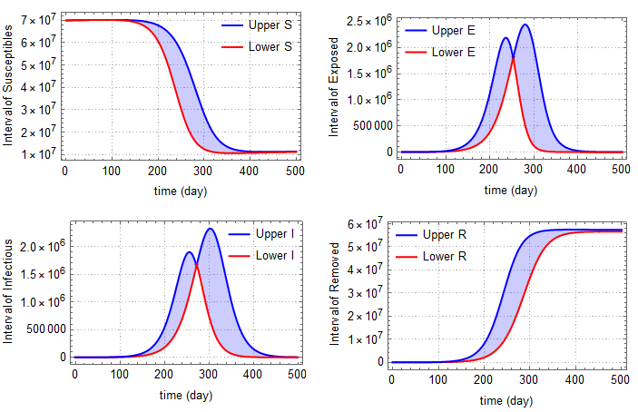
For example, according to this figure we obtained, expected intervals in the population size of compartments at day \(180\)th for our model are as follows:
\begin{eqnarray*} S\left( 180\right) &=&\left[ 6.59804\times 10^{7},6.91713\times 10^{7}\right] , \\ E\left( 180\right) &=&\left[ 193471,574450\right] , \\ I\left( 180\right) &=&\left[ 87797,234169\right] , \\ R\left( 180\right) &=&\left[ 1.04071\times 10^{6},3.74279\times 10^{6}\right] . \end{eqnarray*} It should be noted that, in cases where the exact values of the temporal responses of the process revealed from the model cannot be calculated, this obtained temporal response interval is of course very significant and gives the prediction interval about the current situation.