Long-time solutions for some mixed boundary value problems depicting motions of a class of Maxwell fluids with pressure dependent viscosity

1. Introduction

The study of the motion of a fluid between parallel walls is both of theoretical and practical interest. It was extensively developed due to the various applications in engineering problems. However, very few studies from the existing literature took into consideration the fact that the fluid viscosity does not remain constant at high values of the pressure. The first who remarked this variation of viscosity with the pressure was Stokes in 1845 [1]. During the time experimental investigations (see for instance the book of Bridgman [2] for the pertinent literature prior to 1931, Cutler et al., [3], Johnson and Tewaarwerk [4], Bair and Winer [5] or more recently Bair and Kottke [6] and Prusa et al., [7] have certified this supposition. In elastohydrodynamic lubrication, for instance, the effect of the pressure on viscosity cannot be neglected. In addition, relatively recent Kannan and Rajagopal [8] have remarked that in many motions with practical applications the gravity has a significant influence. Its effects are stronger if the pressure varies along the direction in which the gravity acts.

The first exact steady solutions for isothermal unsteady motions of the incompressible Newtonian fluids (INF) with pressure-dependent viscosity in which the effects of gravity are taken into consideration have been established by Rajagopal [9,10] and Prusa [11]. Analytical expressions of the long-time (permanent or Long) solutions corresponding to the modified Stokes' problems for such fluids with power-law dependence of viscosity on the pressure have been recently determined by Fetecau and Agop [12] and Fetecau and Vieru [13]. Some of them have been already extended to incompressible Maxwell fluids (IMF) of the same type by Fetecau and Rauf [14] and Fetecau et al., [15].

However, all the above mentioned results correspond to boundary value problems in which the velocity is given on the boundary. In practice, there are many situations in which the shear stress is given on a part of the boundary. They lead to mixed boundary value problems. Long-time solutions for such problems describing motions of IFM with power-law dependence of viscosity on the pressure have been determined by Fetecau et al., [16,17]. The purpose of this note is to provide closed-form expressions for the dimensionless velocity, shear stress and normal stress fields corresponding to such motions of a new class of IMF with power-law dependence of viscosity on the pressure. The obtained results have been easy particularized to recover similar solutions for the classical Incompressible Maxwell fluids (CIMF) performing the same motions. The influence of the pressure-viscosity coefficient on the fluid motion were graphically underlined and discussed.

2. Constitutive and governing equations

The constitutive equations of IMF with pressure-dependent viscosity are given by the following relations (see Karra et al., [18] Into above relations T is the Cauchy stress tensor, S is the extra-stress tensor,\(A = L + L^{T}\) is the first Rivlin-Ericksen tensor (L being the gradient of the velocity vector \(v\)), I is the unit tensor, \(\lambda\) is the relaxation time of the fluid, \(\eta( \cdot )\)is the viscosity function and p is the Lagrange multiplier. However, as well as in [18], in the following we shall refer to p as pressure although in the governing equations (1) it is not the mean normal stress. Due to the incompressibility constraint, the next condition, has to be satisfied. Constitutive equations of the form (1) involve the fact that frictional forces exerted by adjacent layers on the fluid depend of the normal force that acts between layers. In the following, we shall consider for the viscosity function \(\eta( \cdot )\)a power-law form having a subunit index, namely where \(\alpha\) is the dimensional pressure-viscosity coefficient and is the fluid viscosity at the reference pressure \(p_{0}\). If the constant \(\alpha = 0\) in Eq. (3), the function \(\eta(p) = \mu\) and the equations (1) reduce to the constitutive equations of CIMF. On the other hand, if \(\lambda = 0\), the equations (1) define an INF with pressure-dependent viscosity. If both \(\alpha\) and \(\lambda\) are zero in these equations, the constitutive equations of classical incompressible Newtonian fluids (CINF) are recovered.

Let us now consider an IMF with power-law dependence of viscosity on the pressure of the form (3) at rest between two infinite horizontal parallel plates at the distance d one of the other. At the moment \(t = 0^{+}\) the lower plate begins to apply a time dependent shear stress

or to the fluid. For, corresponding to INF with pressure-dependent viscosity, the previous expressions tend to the simple forms, where S and are the amplitude, respectively the frequency of the oscillations.

Due to the shear the fluid begins to move and, as well as Karra et al., [18], we are looking for a velocity field and pressure of the form

where is the unit vector lengthways the x-axis of a suitable Cartesian coordinate system x, y and z whose y-axis is perpendicular to the plates. For this velocity field the incompressibility condition (2) is identically satisfied. We also assume that the extra-stress tensor S, as well as the fluid velocity \(v\), is a function of y and t only. The fact that the fluid was at rest up to the initial moment allows us to show that the components \(S_{\text{xz}},S_{\text{yy}},S_{\text{yz}}\) and \(S_{\text{zz}}\) of S are zero while non-trivial normal and shear stresses \(\sigma(y,t) = S_{\text{xx}}(y,t)\), respectively \(\tau(y,t) = S_{\text{xy}}(y,t)\) have to satisfy the following linear differential equations, In the case of conservative body forces but in the absence of a pressure gradient in the flow direction, the balance of linear momentum reduces to the following two relevant partial or ordinary differential equations, in which \(\rho\) is the fluid density and g is the gravitational acceleration. Integrating the second equality (9) from zero to d it results that, Now, eliminating between the equalities (8)\(_{2}\) and (9)\(_{1}\) and bearing in mind the expressions of \(\eta(p)\) and p from the equalities (3), respectively (10), one obtains for the dimensional velocity field \(u(y,t)\) the following partial differential equation, The appropriate initial and boundary conditions are, or again the initial conditions (12) together with the boundary conditions Direct computations show that the solving the ordinary linear differential Eqs (13) and (14) with the initial condition \(\tau(0,0)=0\) leads to expressions of the form (4), respectively (5) for \(\tau(0,t)\)). Consequently, the motion of the IMF in consideration is generated by the lower plate that applies shear stresses of the form (4) or (5) to the fluid. At large values of the time t, these shear stresses can be approximated by the oscillatory expressions, and the fluid motion becomes steady-state or permanent in time. In practice, an important problem for such motions of fluids is to know the need time to reach the steady-state. This is the time after which the transients disappear or can be neglected and the fluid behavior is characterized by the long-time solutions. This is the reason that, in the following, we will establish exact expressions for the dimensionless long-time velocity fields and the adequate shear and normal stresses corresponding to the two motions of IMF with power-law dependence of viscosity on the pressure of the form (3) induced by the lower plate that applies a shear stress of the form (4) or (5) to the fluid.

To do that we introduce the next non-dimensional variables, functions and parameters,

in the previous relations. Dropping out the star notation one obtains the following mixed initial-boundary value problem for the dimensionless velocity field \(u(y,t)\), If the velocity \(u(y,t)\) is determined, the corresponding shear and normal stresses \(\tau(y,t)\) and \(\sigma(y,t)\) can be successively obtained solving the ordinary linear differential equations, Into above relations the non-dimensional constants Re and We defined by, are Reynolds, respectively Weissenberg numbers, is the kinematic viscosity of the fluid and V is a characteristic velocity.

3. Long-time solutions

For distinction, we denote by \(u_{c}(y,t)\), \(\tau_{c}(y,t)\), \(\sigma_{c}(y,t)\) and \(u_{s}(y,t)\), \(\tau_{s}(y,t)\), \(\sigma_{s}(y,t)\) the dimensionless starting solutions corresponding to the two motions of IMF with power-law dependence of viscosity on the pressure induced by the lower plate that applies shear stresses of the form (4), respectively (5) to the fluid. These solutions can be presented as sums of the long-time components \(u_{\text{cp}}(y,t)\), \(\tau_{\text{cp}}(y,t)\), respectively \(u_{\text{sp}}(y,t)\), \(\tau_{\text{sp}}(y,t)\), \(\sigma_{\text{sp}}(y,t)\) and the corresponding transient components. Some time after the motion initiation, the fluid moves according to the starting solutions. After this time, when the transients disappear, the fluid motion is characterized by the long-time solutions which are independent of the initial conditions but satisfy the boundary conditions and the governing equations. In practice, this time is important for the experimental researchers who want to know the required time to touch the steady or permanent state. To determine this time the long-time solutions have to be known and we shall determine them in the following.

3.1. Exact expressions for the long-time velocity fields \(u_{\text{cp}}(y,t)\) and \(u_{\text{sp}}(y,t)\)

In order to determine both components in a simple way and in the same time, let us denote by the dimensionless complex velocity defined by the relation, where i is the imaginary unit. Bearing in mind the relations (17) and (19) it results that has to be solution of the following mixed boundary value problem, Making the change of independent variable, it results that the complex function, has to satisfy the partial differential equation, with the boundary conditions, The form of the boundary conditions (29) and the linearity of the governing Eq. (28) suggest us to look for a solution of the form, Substituting from Eq. (30) in (28) and (29) it results that the complex function has to satisfy the following mixed boundary value problem, The Eq. (31) is an ordinary differential equation of Airy type whose general solution is of the form (see for instance [19, the exercise 34 on the page 251]), where \(C_{1}\) and \(C_{2}\) are arbitrary complex constants and Using the boundary conditions (31)\(_{2}\) and (31)\(_{3}\) we get the function and then Consequently, the complex velocity is given by the relation while the dimensionless velocity fields and have the following expressions, where \(\mathfrak{Re}\) and \(\mathfrak{Im}\) denote the real, respectively the imaginary part of that which follows. As expected, making into above relations, the similar solutions corresponding to the isothermal motions of INF with power-law dependence of viscosity on the pressure of the form (3) induced by the lower plate that applies a shear stress of the form \(S\cos(\omega t)\) or \(S\sin(\omega t)\) to the fluid are recovered [20, Eqs (31) and (32)].

3.2. Exact expressions for the long-time shear stresses \(\tau_{\mathbf{\text{cp}}}(y,t)\) and \(\tau_{\mathbf{\text{sp}}}(y,t)\)

The dimensionless complex shear stress, as it results from the equality (20)\(_{1}\), has to satisfy the linear ordinary differential equation, Based on the same grounds as before, we are looking for a solution of the form, Deriving from Eq. (35) with regard to y, one obtains By substituting \(\tau_{p}(y,t)\) and the derivative of \(u_{p}(y,t)\) with respect to y from Eqs. (40) and (41) respectively, in (39) and following the same way as before, we find that, and therefore, Direct computations clearly show that \(u_{p}(y,t)\) and \(\tau_{p}(y,t)\) given by the equalities (35) and (42) satisfy the partial differential equation (39). The dimensionless long-time frictional forces per unit area exerted by the fluid on the stationary plate are given by the relations,

3.3. Exact expressions for the normal stresses\(\sigma_{\mathbf{\text{cp}}}(y,t)\) and \(\sigma_{\mathbf{\text{sp}}}(y,t)\)

The complex normal stress \(\sigma_{p}(y,t)\) defined by the equality, has to satisfy the linear ordinary equation (see the equality (21)), in which the derivative of \(u_{p}(y,t)\) with regard to y and \(\tau_{p}(y,t)\) are given by the relations (41), respectively (42). Following the same way as before, it is not difficult to show that Consequently, the normal stresses \(\sigma_{\mathbf{\text{cp}}}\mathbf{(y,t)}\) and \(\sigma_{\text{sp}}(y,t)\) have the following expressions Of course, the equality (48) is identically satisfied if \(u_{p}(y,t)\), \(\tau_{p}(y,t)\) and \(\sigma_{p}(y,t)\) are given by the relations (35), (42) and (49) respectively.

4. Limiting cases

In this section, for a check of results that have been previously obtained, some limiting cases are considered and different known results from the existing literature are recovered.

4.1. Case \(\omega \rightarrow 0\); Motion due to an exponential shear stress on the boundary

As we already justified in §2, the motions that have been previously studied are induced by the lower plate that applies a shear stress of the form (4) or (5) to the fluid. Making in Eq. (4), the corresponding motion is due to an exponential shear stress, on the boundary. For differentiation, the dimensionless steady solutions corresponding to this motion will be denoted by \(u_{\text{Ep}}(y)\), \(\tau_{\text{Ep}}(y)\) and \(\sigma_{\text{Ep}}(y)\). Logically speaking, they have to be the limits of \(u_{\text{cp}}(y,t)\), \(\tau_{\mathbf{\text{cp}}}\mathbf{(y,t)}\), respectively \(\sigma_{\mathbf{\text{cp}}}\mathbf{(y,t)}\) when \(\omega \rightarrow 0\), i.e., In order to determine the expressions of \(u_{\text{Ep}}(y)\), \(\tau_{\text{Ep}}(y)\) and \(\sigma_{\text{Ep}}(y)\) in a simple way, let us consider the motion of INF with power-law dependence of viscosity on the pressure of the form (3) produced by the lower plate that applies a constant shear stress S to the fluid. 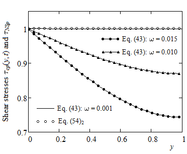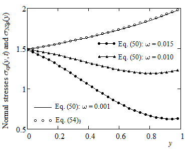Direct computations show that the dimensionless steady solutions corresponding to this last motion are given by the following relations, and Figures 1-3 clearly show that the diagrams of \(u_{\text{cp}}(y,t)\), \(\tau_{\mathbf{\text{cp}}}\mathbf{(y,t)}\) and \(\sigma_{\mathbf{\text{cp}}}\mathbf{(y,t)}\) tend to superpose over those of \(u_{\text{NSp}}(y)\), \(\tau_{\text{NSp}}\), respectively \(\sigma_{\text{NSp}}(y)\) when \(\omega \rightarrow 0\).

Consequently, the solutions \(u_{\text{Ep}}(y)\), \(\tau_{\text{Ep}}\) and \(\sigma_{\text{Ep}}(y)\) are given by the relations,

This is not a surprise because, in the steady case, the governing equations corresponding to two motions of IMF or INF with power-law dependence of viscosity on the pressure as well as the boundary conditions at large values of the time t are identical. In addition, a surprising result consists in the fact that the dimensionless shear stress is constant on the entire flow domain although the corresponding velocity and normal stress are functions of the spatial variable y and the pressure-viscosity coefficient . Furthermore, this constant is even the dimensionless shear stress applied by the lower plate to the INF.

4.2. Case \(\alpha\rightarrow 0\) ; Long-time solutions for CIMF performing the initial motions

Based on some approximations of the standard Bessel functions \(J_{\nu}( \cdot )\)and \(Y_{\nu}( \cdot )\), namely it is not difficult to show that the complex fields \(u_{p}(y,t)\), \(\tau_{p}(y,t)\) and \(\sigma_{p}(y,t)\) can be approximated by the following expressions, for small enough values of the non-dimensional pressure-viscosity coefficient \(\alpha\). Now, using the Maclaurin series expansions of the expressions \(\lbrack 1 + \alpha(1 - y)\rbrack^{3/4}\) and \((1 + \alpha)^{3/4}\) in the approximations (57)-(59) and then the identities, and taking the limit of the obtained results for \(\alpha\rightarrow 0\) one obtains the dimensionless complex velocity, shear stress and normal stress fields, corresponding to the CIMF performing the initial motions. Into above relations the complex constant Consequently, the dimensionless velocity fields \(u_{\text{Ccp}}(y,t)\), \(u_{\text{Csp}}(y,t)\) and the adequate shear and normal stresses \(\tau_{\text{Ccp}}(y,t)\), \(\tau_{\text{Csp}}(y,t)\), \(\sigma_{\text{Ccp}}(y,t)\), \(\sigma_{\text{Csp}}(y,t)\) corresponding to the these motions of CIMF are given by the relations (see Fetecau et al., [17, Eqs. (70)-(75)]

4.3. Case \(\alpha\) and \(\omega\rightarrow 0\); Motion of CIMF due to an exponential shear stress on the boundary

Making \(\alpha \rightarrow 0\) in Eqs. (55) or \(\omega \rightarrow 0\) in (65), (67) and (69) one recovers the dimensionless steady solutions [17, Eqs. (84)-(86)], corresponding to the isothermal motion of CIMF produced by the lower plate that applies an exponential shear stress \(\lbrack 1 - \exp( - t/\lambda)\rbrack S\) to the fluid. The first two solutions, as expected, are identical to the steady solutions \(u_{\text{CNSp}}(y)\) and \(\tau_{\text{CNSp}}\) corresponding to the isothermal motion of CINF generated by the lower plate that applies a constant shear stress S to the fluid while the corresponding normal stress \(\sigma_{\text{CNSp}} = 0\).

5. Some numerical results and conclusions

Generally, exact solutions corresponding to specific boundary value problems describe the behavior of a material subject to some deformations or motions. In addition, they can be used to verify various numerical schemes that are developed to study more complex problems. In the present work are established analytical expressions for the dimensionless long-time velocities and the adequate normal and shear stresses corresponding to isothermal motions of IMF with power-law dependence of viscosity on the pressure. The fluid motion, between two infinite horizontal parallel plates, is generated by the lower plate that applies time-dependent shear stresses to the fluid. Consequently, contrary to what is usually assumed in the existing literature, the shear stress is prescribed on a part of the boundary. Prescribing the shear stress on the plate is the same to give the force applied in order to move it.

Obtained solutions are presented in simple forms in terms of standard Bessel functions. For a check of their corrections, the dimensionless steady solutions \(u_{\text{NSp}}(y)\),\(\tau_{\text{NSp}}\) and \(\sigma_{\text{NSp}}(y)\) corresponding to the isothermal motion induced by the lower plate that applies a constant shear stress S to an INF with power-law dependence of viscosity on the pressure have been used. More exactly, by means of Figures 1-3, the convergence of long-time solutions , and to these solutions has been graphically proved. In this way, as it was to be expected, we showed that the dimensionless steady solutions \(u_{\text{Ep}}(y)\), \(\tau_{\text{Ep}}\) and \(\sigma_{\text{Ep}}(y)\) corresponding to the isothermal motion generated by the lower plate that applies an exponential shear stress \(\lbrack 1 - \exp( - t/\lambda)\rbrack S\) to an IMF with power-law dependence of viscosity on the pressure are identical to \(u_{\text{NSp}}(y)\),\(\tau_{\text{NSp}}\), respectively \(\sigma_{\text{NSp}}(y)\).

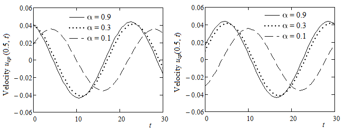
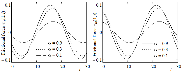
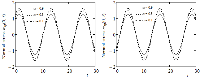
Finally, in order to emphasize some physical insight of results that have been here obtained, Figures 4-10 have been depicted for different values of the dimensionless pressure-viscosity coefficient and of the spatial variable y. The time variation of the mid plane velocities \(u_{\text{cp}}(0.5,t),u_{\text{sp}}(0.5,t)\), of frictional forces per unit area \(\tau_{\text{cp}}(1,t),\tau_{\text{sp}}(1,t)\) exerted by the fluid on the fixed plate and of the normal stresses \(\sigma_{\text{cp}}(0,t)\) and \(\sigma_{\text{sp}}(0,t)\) on the moving plate are presented in Figures 4-6 at increasing values of and fixed values of the other parameters. The oscillatory characteristic features of these entities of physical interest, as well as the phase difference between solutions corresponding to motions due to shear stresses of the form (4) or (5) on the boundary, are clearly visualized. From Figures 4 and 5 it also results that the larger pressure-viscosity coefficient the larger amplitude of velocity and shear stress oscillations. An opposite result appears in the case of normal stresses.

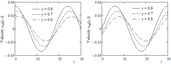
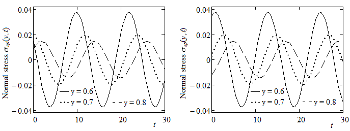
Figures 7-9 together present the time variations of \(u_{\text{cp}}(y,t)\) and \(u_{\text{sp}}(y,t)\),\(\tau_{\mathbf{\text{cp}}}\mathbf{(y,t)}\) and \(\tau_{\text{sp}}(y,t)\), respectively \(\sigma_{\text{cp}}(y,t)\) and \(\sigma_{\mathbf{\text{sp}}}\mathbf{(y,t)}\) at increasing values of the spatial variable y. As expected, the oscillations' amplitude corresponding to the fluid velocity and shear stress diminishes for increasing values of y while the amplitude of normal stresses is an increasing function with respect to this variable. Consequently, the fluid velocity and the corresponding shear stress in absolute value are higher in the vicinity of the moving plate. 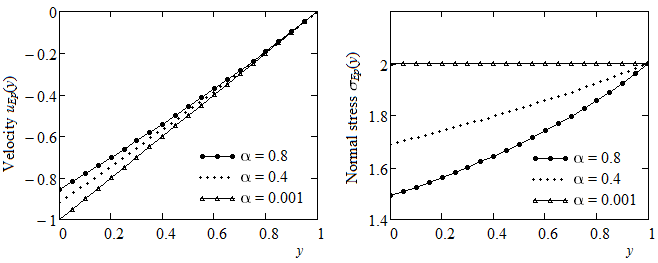Last Figure 10 presents the variations of \(u_{\text{Ep}}(y)\) and \(\sigma_{\text{Ep}}(y)\) at increasing values of the pressure-viscosity coefficient \(\alpha\). The fluid velocity in absolute value, as well as the normal stress, is a decreasing function of \(\alpha\). This is possible because the fluid viscosity increases for growing values of \(\alpha\) and its velocity decreases. Both entities smoothly increase from minimum values on the lower plate to the values zero, respectively two on the upper plate.

The significant outcomes that have been obtained by means of the present study are:

• Two isothermal motions of some IMF with power-law dependence of viscosity on the pressure between parallel plates were investigated when the gravity effects are taken into consideration.
• Analytical expressions for the dimensionless long-time solutions corresponding to these motions were established when the lower plate applies time-dependent shear stresses to the fluid.
• As a check of their corrections, the solutions of CIMF performing same motions have been recovered as limiting cases of present results using appropriate approximations of Bessel functions.
• Oscillatory behavior of these motions, phase difference between them and the influence of pressure-viscosity coefficient on the obtained solutions is graphically brought to light and discussed.
• Similar solutions for the motion of same fluids generated by the lower plate that applies an exponential shear stress \(\lbrack 1 - \exp( - t/\lambda)\rbrack S\) to the fluid have been also determined.
• Steady shear stress corresponding to this motion is constant on the entire flow domain although the corresponding velocity and normal stress are functions of y and . This constant is even the non-dimensional shear stress applied to the fluid by the lower plate.

Author Contributions:

All authors contributed equally in this paper. All authors read and approved the final version of this paper.

Conflicts of Interest:

The authors declare no conflict of interest.

Data Availability:

All data required for this research is included within this paper.

Funding Information:

No funding is available for this research.