Steady-state solutions for modified Stokes’ second problem of Maxwell fluids with power-law dependence of viscosity on the pressure

1. Introduction

The motion of fluid over an infinite plate oscillating in its plane is termed as Stokes' second problem by Schlichting [1]. It is termed as the modified Stokes' second problem by Rajagopal et al., [2] if the fluid is bounded by two parallel walls. Both motions are important from the theoretical and practical point of view because they appear in many applied problems, such as flows in vibrating media. If the fluid has been at rest up to the initial moment, its motion becomes steady in time and a very important problem for experimentalists is to know the time after which the steady or permanent state is obtained. To determine this time, at least the steady-state (permanent or long-time) solutions have to be known.

The fact that the fluid viscosity could depend on the pressure was early enough suggested by Stokes [3] and the experimental investigations (see for instance Bridgman [4], Cutler et al., [5], Johnson and Tewaarwerk [6], Bair and Winer [7] and Prusa et al., [8] have certified this supposition. For instance, in elastohydrodynamic lubrication problems, the effects of pressure on viscosity cannot be neglected. Concerning the importance of the pressure- dependent viscosity in steady motions of incompressible fluids, we recommend the paper of Huilgol, and You [9]. On the other hand, Kannan and Rajagopal [10] remarked that gravity has a notable influence in different motions with engineering applications. Its effects are more pronounced if the pressure alters along the direction in which the gravity acts. First exact solutions for steady motions of incompressible Newtonian fluids with pressure-dependent viscosity in which the influence of gravity is taken into consideration are those of Rajagopal [11,12]. Interesting steady and starting solutions for the modified Stokes' problems of Newtonian fluids with pressure-dependent viscosity have also been established by Prusa [13], respectively Rajagopal et al., [12] when the gravity effects are taken into consideration. Recently, permanent solutions corresponding to motions of incompressible Newtonian fluids with power-law dependence of viscosity on the pressure have been determined by Fetecau, and Agop [14], Fetecau and Vieru [15], and Fetecau and Rauf [16]. Some of them have already been extended to incompressible Maxwell fluids (IMF) of the same type [17,18,19].

The goal of this work is to provide closed-form expressions for the steady-state solutions corresponding to the modified Stokes' second problem and the simple Couette flow for a class of IMF with power-law dependence of viscosity on the pressure. Analytical expressions are established for the dimensionless velocity fields and the corresponding nontrivial shear and normal stresses. For a check of their correctness, it was graphically proved that the diagrams of the solutions corresponding to the motion induced by cosine oscillations of the plate are almost identical to those of the simple Couette flow if the oscillations' frequency is small enough. In addition, similar solutions for ordinary IMF and incompressible Newtonian fluids (IMF) with power-law dependence of viscosity on the pressure performing the same motions are obtained as limiting cases of general results. The influence of the main parameters on the fluid motion is graphically underlined and discussed.

2. Formulation of the problem

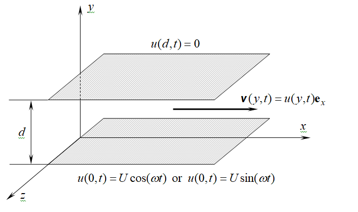
Let us consider an IMF with pressure-dependent viscosity at rest between two infinite horizontal parallel plates at the distance d one of the other as it is illustrated in Figure 1. Its constitutive equations, as they have been presented by Karra et al., [20], are given by the following relations Here T is the stress tensor, S the extra-stress tensor, I the unit tensor, L is the gradient of the velocity vector v and \(\lambda\) is the relaxation time of the fluid. The viscosity function \(\eta( \cdot )\) to be here used has the following power-law form

where \(\alpha\) is the pressure-viscosity coefficient and \(\mu\) is the fluid viscosity at the reference pressure \(p_{0}\). We shall refer to the Lagrange multiplier p as pressure although, for such fluids, it is not the mean normal stress [20].

If \(\lambda \rightarrow 0\) in the equality \((1)_{2}\), the new constitutive equations (1) define incompressible Newtonian fluids (INF) with pressure-dependent viscosity. If \(\alpha = 0\) in Eq. (2) \(\eta(p) = \mu\) and the adequate constitutive equations (1) correspond to ordinary IMF. The fact that \(\eta(p) \rightarrow \infty\) for \(p \rightarrow \infty\) is in accordance with a property that have been experimentally confirmed.

At the moment \(t = 0^{+}\) the lower plate begins to oscillate in its plane according to

where \( e_{x}\) is the unit vector along the x-axis of a suitable Cartesian coordinate system x, y, and z whose y-axis is perpendicular to the plates while U and \(\omega\) are the amplitude, respectively the frequency of the oscillations. Due to the shear the fluid begins to move and, as well as Karra et al., [20], we are looking for a velocity field and pressure of the form Assuming that the extra-stress tensor S, as well as the fluid velocity v is also a function of y and t only and using the fact that the fluid was at rest up to the moment \(t = 0\), it is not difficult to show that the components \(S_{\text{xz}},\ S_{\text{yy}},\ S_{\text{yz}}\ \)and \(S_{\text{zz}}\) of the extra-stress tensor S are zero while the non-trivial shear and normal stresses \(\tau(y,t) = S_{\text{xy}}(y,t)\), respectively \(\sigma(y,t) = S_{\text{xx}}(y,t)\) have to satisfy the following linear differential equations In the absence of a pressure gradient in the flow direction, the balance of momentum reduces to the next two relevant partial or ordinary differential equations while the incompressibility condition is identically satisfied. Into above relations \(\rho\) is the density of the fluid and g is the gravitational acceleration. Integrating the second equation with respect to y between the limits 0 and d, it results that Now, eliminating the shear stress \(\tau(y,t)\) between the equalities \((5)_{1}\) and \((6)_{1}\) and bearing in mind the expressions of \(\eta(p)\) and p from the equalities (2), respectively (7) one obtains for the dimensional velocity field \(u(y,t)\) the following initial and boundary value problem As soon as the fluid velocity \(u(y,t)\) is known, the corresponding shear and normal stresses \(\tau(y,t)\) and \(\sigma(y,t)\) can be determined from the next linear differential equations Introducing the following non-dimensional variables, functions and parameters in the governing equations (8)-(12) and dropping out the star notation, one obtains the next dimensionless initial and boundary value problem for the velocity field \(u(y,t)\) and the linear differential equations with initial conditions for the shear and normal stresses. Into above relations \(\text{Re} = Ud/\nu\) and \(\text{We}\ = \lambda U/d\) are Reynolds, respectively Weissenberg dimensionless numbers and \(\nu = \mu/\rho\) is the kinematic viscosity of the fluid.

3. Solution of the problem

In order to evade possible confusions, we denote by \(u_{c}(y,t)\), \(\tau_{c}(y,t)\), \(\sigma_{c}(y,t)\) and \(u_{s}(y,t)\), \(\tau_{s}(y,t)\), \(\sigma_{s}(y,t)\) the dimensionless starting solutions corresponding to the two motions induced by cosine, respectively sine oscillations of the lower plate. These solutions can be represented as sums of their permanent and transient components, namely Up to the moment \(t = t_{\text{cp}}\) or \(t = t_{\text{sp}}\) which is the time to reach the permanent state, the fluid behavior is described by the starting solutions. After this time, when the absolute values of the transient components are small enough and can be neglected, the fluid moves according to the permanent solutions \(u_{\text{cp}}(y,t)\), \(\tau_{\text{cp}}(y,t)\), \(\sigma_{\text{cp}}(y,t)\), respectively \(u_{\text{sp}}(y,t)\), \(\tau_{\text{sp}}(y,t)\), \(\sigma_{\text{sp}}(y,t)\) which are independent of the initial conditions but satisfy the boundary conditions and governing equations. In order to determine this time, which in practice is important for experimentalists, it is sufficient to know analytical expressions for the permanent solutions. To find these solutions in the same time for both motions, we define the non-dimensional complex velocity, shear stress and normal stress by the next relations where i is the imaginary unit.

The complex velocity \(u_{p}(y,t)\) has to satisfy the following boundary value problem

while the complex stresses \(\tau_{p}(y,t)\) and \(\sigma_{p}(y,t)\) have to be solutions of the ordinary linear differential equations Bearing in mind the form of the boundary conditions (23) and the linearity of the governing equations (22) and (24), we are looking for solutions of the form where \(V(y)\), \(T(y)\) and \(S(y)\) are complex functions.

3.1. Calculation of the complex velocity \(u_{p}(y,t)\)

By substituting \(u_{p}(y,t)\) from Eq. \((26)_{1}\) in (22) and (23), one obtains for the function \(V(y)\) the following ordinary differential equation with boundary conditions where \(\gamma = \sqrt{- i\omega Re(1 + i\omega\text{We}\ )}\). Now, making the next changes of the independent spatial variable y and the unknown function \(V(y)\) one obtains for the function \(W(z)\) the following suitable ordinary differential equation with the next boundary conditions Making a new change of independent variable, namely \(z = \alpha r/(3\gamma)\), one attains to an Euler-Bessel equation whose well known general solution allow us to determine where \(a = 3\gamma/\alpha,\ \ b = a\ \sqrt[3]{1 + \alpha}\) while \(J_{1/2}( \cdot )\) and \(Y_{1/2}( \cdot )\) are Bessel standard functions of the order 1/2. By substituting \(W(z)\) in \((28)_{2}\) and the obtained result in \((26)_{1}\), it results that Consequently, the permanent velocities \(u_{\text{cp}}(y,t)\) and \(u_{\text{sp}}(y,t)\) are given by the relations where \(\mathfrak{R}e\) and Im denotes the real, respectively the imaginary part of that which follows. Of course, the boundary conditions (16) are clearly satisfied.

3.2. Calculation of the complex stresses \(\tau_{p}(y,t)\) and \(\sigma_{p}(y,t)\)

By derivation of the equality (32) with respect to y one obtains Substituting the expression of \(\partial u_{p}(y,t)/\partial y\) in Eq. (24) and bearing in mind the relation \((26)_{2}\), it results for the complex shear stress \(\tau_{p}(y,t)\) the expression Consequently, the permanent shear stresses \(\tau_{\text{cp}}(y,t)\) and \(\tau_{\text{sp}}(y,t)\) have the forms Direct computations show that the complex normal stress \(\sigma_{p}(y,t)\) has the form and the permanent solutions \(\sigma_{\text{cp}}(y,t)\) and \(\sigma_{\text{sp}}(y,t)\) can be immediately written as being Finally, it is worth pointing out the fact that the similar dimensionless solutions corresponding to INF with power-law dependence of viscosity on the pressure performing the same motions are immediately obtained taking \(\text{We} = 0\) in Eqs. (33), (34), (37), (38) (40) and (41). Into above relations \(c = 3\sqrt{- i\omega\text{Re}}\ /\alpha\) and \(d = c\sqrt[{\ 3}]{1 + \alpha}\).

4. Results' validation

In order to validate the correctness of results which have been here obtained, we shall compare their limits for \(\alpha \rightarrow 0\) or \(\omega \rightarrow 0\) with known results from the literature, respectively with the similar solutions corresponding to the simple Couette flow of the same fluids.

4.1. Case \(\alpha \rightarrow 0\); Modified Stokes' second problem for ordinary IMF

Using convenient asymptotic approximations of the Bessel functions, namely it is not difficult to show that for small enough values of the pressure-viscosity coefficient \(\alpha\) permanent solutions \(u_{\text{cp}}(y,t)\) and \(u_{sp}(y,t)\) can be approximated by the following relations Now, substituting the Maclaurin series expansions of \(\lbrack 1 + \alpha(1 - y)\rbrack^{1/3}\) and \((1 + \alpha)^{1/3}\) in the previous relations and taking their limits for \(\alpha \rightarrow 0\), one recovers the permanent solutions corresponding to ordinary IMF performing the same motions, namely Indeed, using the known relations \(sin(\text{iz}) = isinh(z)\) and \(\sqrt{- i} = - i\sqrt{i}\), it results that where \(\delta = \sqrt{i\omega Re(1 + i\omega We)}\). As expected, the expression of \(u_{\text{Osp}}(y,t)\) from Eq. \((52)_{2}\) is identical to that obtained by Fetecau et al., [21, Eq. (36) with \(K = 0\)].

Similar computations show that the stresses \(\tau_{\text{cp}}(y,t)\), \(\tau_{\text{sp}}(y,t)\), \(\sigma_{\text{cp}}(y,t)\) and \(\sigma_{\text{sp}}(y,t)\) can be approximated by the following relations:

Using again the previous identities and the fact that \(\cos(\text{iz}) = \cosh(z)\) in the equalities (53), (54), (55) and (56) and taking their limits for \(\alpha \rightarrow 0\), it results that As it was to be expected, the expression of \(\tau_{\text{Osp}}(y,t)\) from Eq. (58) is identical to that obtained by Fetecau et al., [21, Eq. (42) with \(K = 0\)] by a different technique.

4.2. Case \(\omega \rightarrow 0\); Simple Couette flow of IMF with power-law dependence of viscosity on the pressure

The dimensionless permanent solutions corresponding to the simple Couette flow of IMF with power-law dependence of the form (2) of velocity on the pressure, namely

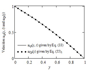
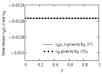
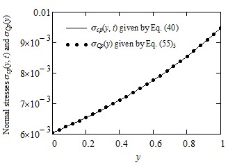
can be easily determined successively solving the corresponding governing equations. As expected, Figures 2-4 show that the diagrams of \(u_{\text{cp}}(y,t)\), \(\tau_{\text{cp}}(y,t)\) and \(\sigma_{\text{cp}}(y,t)\) are almost identical to those of \(u_{\text{Cp}}(y),\text{    }\tau_{\text{Cp}}\), respectively \(\sigma_{\text{Cp}}(y)\) if the frequency \(\omega\) of the oscillations as well as the product \(\omega\)t is small enough. A surprising result is the fact that the permanent shear stress \(\tau_{\text{Cp}}\) corresponding to the simple Couette flow of such fluids is constant on the whole flow domain although the fluid velocity \(u_{\text{Cp}}(y)\) and the corresponding normal stress \(\sigma_{\text{Cp}}(y)\) are functions of the spatial variable y. However, this shear stress as well as the fluid velocity and the normal stress depend on the pressure-viscosity coefficient.

4.3. Case \(\alpha \rightarrow 0\) and \(\omega \rightarrow 0\) Simple Couette flow of ordinary IMF

Finally, making \(\omega \rightarrow 0\) in Eqs. \((52)_{1}\), (57) and (59) or \(\alpha \rightarrow 0\) in Eqs. (61) one obtains the steady solutions corresponding to the simple Couette flow of ordinary IMF, namely The first two steady solutions \(u_{\text{OCp}}(y)\) and \(\tau_{\text{OCp}}\) are identical to the similar solutions \(u_{\text{ONCp}}(y)\), respectively \(\tau_{\text{ONCp}}\) corresponding to the simple Couette flow of ordinary INF and the expression of the velocity field given by Eq. (62) has been previously obtained by Erdogan [22]. In exchange, as it results from Eq. (64), the steady normal stress corresponding to the same motion of ordinary incompressible Newtonian fluids is zero.

5. Some numerical results and conclusions

The main purpose of this note is to offer a simple alternative for those who want to find the necessary time to reach the permanent state (steady state) corresponding to the modified Stokes' second problem of some IMF with power-law dependence of viscosity on the pressure. To do that, exact expressions are established for the dimensionless permanent solutions corresponding to the velocity field and the non-trivial shear and normal stresses. The required time to touch the permanent state can be graphically determined by comparing these solutions with the corresponding starting solutions (numerical solutions). It is the time after which the diagrams of starting solutions superpose over those of the permanent solutions and the fluid behavior is characterized by the steady-state solutions only.

For completion, as well as for a check of the correctness of results that have been here obtained; exact expressions are also determined for the similar solutions correspond to the simple Couette flow of the same fluids. Figures 2-4, as it was to be expected, clearly show that for a small enough value of the oscillations' frequency \(\omega\) the diagrams of solutions \(u_{\text{cp}}(y,t)\), \(\tau_{\text{cp}}(y,t)\) and \(\sigma_{\text{cp}}(y,t)\) are almost identical to those of the simple Couette flow \(u_{\text{Cp}}(y)\), \(\tau_{\text{Cp}}\) and \(\sigma_{\text{Cp}}(y)\), respectively. The dimensionless steady state solutions corresponding to the ordinary IMF performing the same motions, as well as those of the INF with power-law dependence of viscosity on the pressure is obtained as limiting cases of the initial solutions.

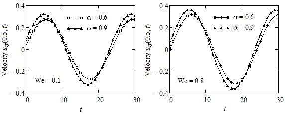
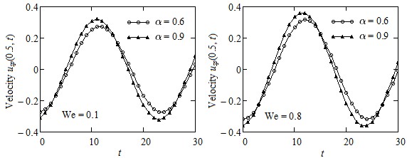
In order to bring to light the influence of Weissenberg number We and of the pressure-viscosity coefficient \(\alpha\) on the fluid motion Figures 5 and 6 and Table 1 have been included here. In these figures the time variations of the mid plane velocities \(u_{\text{cp}}(0.5,t)\) and \(u_{\text{sp}}(0.5,t)\) are presented at distinct values of the two parameters. Oscillatory specific features of the two motions and the phase difference between them are clearly visualized. It also results that the order of magnitude of the oscillations' amplitude for common values of the parameters is the same for both movements and the smaller values of pressure-viscosity coefficient \(\alpha\) or We the smaller the oscillations' amplitude. Consequently, the fluid decelerates for decreasing values of the two parameters, and the lowest velocity corresponds to the ordinary IMF, respectively the INF with pressure-dependent viscosity. As regards the Weissenberg number We, as it was proved by Poole [23], it represents the ratio of elastic to viscous forces. Therefore, at the same elastic properties of the fluid, a decline of We means an increase of viscous forces, which implies a decrease of the fluid velocity. In Table 1, for completion, numerical values of the dimensionless steady velocity \(u_{\text{Cp}}(y)\) corresponding to the simple Couette flow of IMF with power-law dependence of viscosity on the pressure are provided at three values of the pressure-viscosity coefficient \(\alpha\) and different values of the spatial variable y. The fluid velocity, as before, grows for increasing values of \(\alpha\).

Table 1.

y	\(u_{Cp}(y)\)
	\(\alpha=0.2\)	\(\alpha=0.5\)	\(\alpha=0.9\)
0	1	1	1
0.1	0.910	0.921	0.932
0.2	0.819	0.839	0.859
0.3	0.725	0.753	0.780
0.4	0.629	0.662	0.696
0.5	0.530	0.567	0.605
0.6	0.430	0.466	0.506
0.7	0.326	0.360	0.398
0.8	0.220	0.247	0.279
0.9	0.112	0.128	0.147
1	0	0	0

The main results that have been obtained by means of the present study are:

• Exact expressions have been established for the steady-state solutions of the modified Stokes' second problem of IMF with power-law dependence of viscosity on the pressure.
• Oscillatory behavior of the two motions and the influence of Weissenberg number and the pressure-viscosity coefficient on fluid velocity was graphically underlined and discussed.
• Similar solutions corresponding to the same problem of ordinary IMF and of INF with power-law dependence of viscosity on the pressure have been obtained as limiting cases of the present results using suitable asymptotic approximations of Bessel functions.
• Steady solutions for the simple Couette flow of IMF with power-law dependence of viscosity on the pressure have been also determined and the convergence of \(u_{\text{cp}}(y,t)\), \(\tau_{\text{cp}}(y,t)\) and \(\sigma_{\text{cp}}(y,t)\) to these solutions was graphically proved when \({ \omega \rightarrow}\mathbf{0}\).
• The shear stress \(\tau_{\text{Cp}}\) corresponding to this motion is constant on the entire flow domain although the velocity \(u_{\text{Cp}}(y)\) and normal stress \(\sigma_{\text{Cp}}(y)\) are functions of the spatial variable y.

Acknowledgments

The authors would like to thank reviewers for their careful assessment, valuable suggestions and comments regarding the initial version of the manuscript.

Conflicts of Interest: 

"The author declares no conflict of interest."

References

Schlichting, H. (1968). Boundary Layer Theory. McGraw-Hill, Singapore. [Google Scholor]
Rajagopal, K. R., Saccomandi, G., & Vergori, L. (2013). Unsteady flows of fluids with pressure dependent viscosity. Journal of Mathematical Analysis and Applications, 404(2), 362-372. [Google Scholor]
Stokes, G. G. (2007). On the theories of the internal friction of fluids in motion, and of the equilibrium and motion of elastic solids.
Transactions of the Cambridge Philosophical Society, 8, 287-305, 1845. [Google Scholor]
Bridgman, P. W. (1931). The Physics of High Pressure. The MacMillan Company, New York.
[Google Scholor]
Cutler, W. G., McMickle, R. H., Webb, W., & Schiessler, R. W. (1958). Study of the compressions of several high molecular weight hydrocarbons. The Journal of Chemical Physics, 29(4), 727-740. [Google Scholor]
Johnson, K. L., & Tevaarwerk, J. L. (1977). Shear behaviour of elastohydrodynamic oil films. Proceedings of the Royal Society of London. A. Mathematical and Physical Sciences, 356(1685), 215-236. [Google Scholor]
Bair, S., & Winer, W. O. (1992). The high pressure high shear stress rheology of liquid lubricants. Journal of Tribology, 114, 1-13. [Google Scholor]
Pruša, V., Srinivasan, S., & Rajagopal, K. R. (2012). Role of pressure dependent viscosity in measurements with falling cylinder viscometer. International Journal of Non-Linear Mechanics, 47(7), 743-750. [Google Scholor]
Huilgol, R. R., & You, Z. (2006). On the importance of the pressure dependence of viscosity in steady non-isothermal shearing flows of compressible and incompressible fluids and in the isothermal fountain flow. Journal of non-newtonian fluid mechanics, 136(2-3), 106-117. [Google Scholor]
Kannan, K., & Rajagopal, K. R. (2005). Flows of fluids with pressure dependent viscosities between rotating parallel plates. In: P. Fergola
et al. (Eds.), New Trends in Mathematical Physics, World Scientific, Singapore. [Google Scholor]
Rajagopal, K. R. (2004). Couette flows of fluids with pressure dependent viscosity. International Journal of Applied Mechanics and Engineering, 9(3), 573-585. [Google Scholor]
Rajagopal, K. R. (2008). A semi-inverse problem of flows of fluids with pressure-dependent viscosities. Inverse Problems in Science and Engineering, 16(3), 269-280. [Google Scholor]
Pruša, V. (2010). Revisiting Stokes first and second problems for fluids with pressure-dependent viscosities. International Journal of Engineering Science, 48(12), 2054-2065. [Google Scholor]
Fetecau, C., & Agop, M. (2020). Exact solutions for oscillating motions of some fluids with power-law dependence of viscosity on the pressure. Annals of the Academy of Romanian Scientists: Series on Mathematics and its Applications, 12, 295-311. [Google Scholor]
Fetecau, C., & Vieru, D. (2020). Exact solutions for unsteady motion between parallel plates of some fluids with power-law dependence of viscosity on the pressure. Applications in Engineering Science, 1, 100003, https://doi.org/10.1016/j.apples.2020.100003. [Google Scholor]
Fetecau, C., Rauf, A., Qureshi, T. M., & Khan, M. (2020). Permanent solutions for some oscillatory motions of fluids with power-law dependence of viscosity on the pressure and shear stress on the boundary. Zeitschrift für Naturforschung A, 75(9), 757-769. [Google Scholor]
Fetecau, C., & Rauf, A. (2021). Permanent solutions for some motions of UCM uids with power-law dependence of viscosity on the pressure. Studia Universitatis Babes-Bolyai, Mathematica, 66(1), 197-209. [Google Scholor]
Fetecau, C.,Vieru, D., Rauf, A., & Qureshi, T. M.(2021). Steady-state solutions for some motions of Maxwell fluids with pressure-dependence of viscosity. Journal of Mathematical Sciences: Advances and Applications, 68, 1-28. [Google Scholor]
Fetecau, C., Qureshi, T. M., Rauf, A., & Vieru, D. (2022). On the modified stokes second problem for maxwell fluids with linear dependence of viscosity on the pressure. Symmetry, 14(2), Article No. 219, https://doi.org/10.3390/sym14020219.[Google Scholor]
Karra, S., Pruša, V., & Rajagopal, K. R. (2011). On Maxwell fluids with relaxation time and viscosity depending on the pressure. International Journal of Non-Linear Mechanics, 46(6), 819-827. [Google Scholor]
Fetecau, C., Ellahi, R., & Sait, S. M. (2021). Mathematical analysis of Maxwell fluid flow through a porous plate channel induced by a constantly accelerating or oscillating wall. Mathematics, 9(1), Article No. 90, https://doi.org/10.3390/math9010090. [Google Scholor]
Erdogan, M. E. (2002). On the unsteady unidirectional flows generated by impulsive motion of a boundary or sudden application of a pressure gradient. International Journal of Non-Linear Mechanics, 37(6), 1091-1106. [Google Scholor]
Poole, R. J. (2012). The deborah and weissenberg numbers. Rheology Bulletin, 53(2), 32-39. [Google Scholor]