Open Access Full-Text PDF

Engineering and Applied Science Letters

Computing Degree-Based Topological Indices of Jahangir Graph

Wei Gao, Asima Asghar, Waqas Nazeer\(^1\)
School of Information Science and Technology, Yunnan Normal University, Kunming 650500, China.; (W.G)
Department of Mathematics, The University of Lahore, Pakpattan Campus, Pakpattan 57400, Pakistan.; (A.A)
Division of Science and Technology, University of Education, Lahore 54000, Pakistan.;(W.N)
\(^{1}\)Corresponding Author;  nazeer.waqas@ue.edu.pk

Copyright © 2018 Wei Gao, Asima Asghar and Waqas Nazeer. This is an open access article distributed under the Creative Commons Attribution License, which permits unrestricted use, distribution, and reproduction in any medium, provided the original work is properly cited.

Abstract

Topological indices are numerical numbers associated with a graph that helps to predict many properties of underlined graph. In this paper we aim to compute multiplicative degree based topological indices of Jahangir graph.

Index Terms:

Zagreb index; Randic index; Polynomial; Degree; Graph.

1. Introduction

The study of topological indices, based on distance in a graph, was effectively employed in 1947, in chemistry by Weiner [1]. He introduced a distance-based topological index called the Wiener index to correlate properties of alkenes and the structures of their molecular graphs.

Topological indices play a vital role in computational and theoretical aspects of chemistry in predicting material properties [2, 3, 4, 5, 6, 7, 8]. Several algebraic polynomials have useful applications in chemistry [9, 10]. A graph \(G\) is an ordered pair \((V,E)\), where \(V\) is the set of vertices and \(E\) is the set of edges. A path from a vertex \(v\) to a vertex \(w\) is a sequence of vertices and edges that starts from \(v\) and stops at \(w\). The number of edges in a path is called the length of that path.

A graph is said to be connected if there is a path between any two of its vertices. The distance \(d(u,v)\) between two vertices \(u\), \(v\) of a connected graph \(G\) is the length of a shortest path between them. Graph theory is contributing a lion's share in many areas such as chemistry, physics, pharmacy, as well as in industry [11]. We will start with some preliminary facts.

The first and second multiplicative Zagreb indices [12] are defined as \begin{equation} MZ_{1}(G)=\prod\limits_{u\in V(G)}(d_{u})^{2}, \end{equation} \begin{equation} MZ_{2}(G)=\prod\limits_{uv\in E(G)}d_{u}. d_{u}, \end{equation} and the Narumi-Kataymana index [13] is defined as \begin{equation} NK(G)=\prod\limits_{u\in V(G)}d_{u}, \end{equation} Like the Wiener index, these types of indices are the focus of considerable research in computational chemistry [14, 15, 16, 17]. For example, in 2011, Gutman [14] characterized the multiplicative Zagreb indices for trees and determined the unique trees that obtained maximum and minimum values for \(M_{1}(G)\) and \(M_{2}(G)\). Wang et al. [17] define the following index for k-trees, \begin{equation} W^{s}_{1}(G)=\prod\limits_{u\in V(G)}(d_{u})^{s}. \end{equation} Notice that \(s=1,2\) is the Narumi-Katayama and Zagreb index, respectively. Based on the successful consideration of multiplicative Zagreb indices, Eliasi et al. [18] continued to define a new multiplicative version of the first Zagreb index as \begin{equation} MZ^{\ast}_{1}(G)=\prod\limits_{uv\in E(G)}(d_{u}+d_{u}), \end{equation} Furthering the concept of indexing with the edge set, the first author introduced the first and second hyper-Zagreb indices of a graph [19]. They are defined as \begin{equation} HII_{1}(G)=\prod\limits_{uv\in E(G)}(d_{u}+d_{u})^{2}, \end{equation} \begin{equation} HII_{2}(G)=\prod\limits_{uv\in E(G)}(d_{u}.d_{u})^{2}, \end{equation} In [20] Kulli et al. defined the first and second generalized Zagreb indices \begin{equation} MZ^{a}_{1}(G)=\prod\limits_{uv\in E(G)}(d_{u}+d_{u})^{a}, \end{equation} \begin{equation} MZ^{a}_{2}(G)=\prod\limits_{uv\in E(G)}(d_{u}.d_{u})^{a}, \end{equation} Multiplicative sum connectivity and multiplicative product connectivity indices [21] are define as: \begin{equation} SCII(G)=\prod\limits_{uv\in E(G)}\frac{1}{(d_{u}+d_{u})}, \end{equation} \begin{equation} PCII(G)(G)=\prod\limits_{uv\in E(G)}\frac{1}{(d_{u}.d_{u})}, \end{equation} Multiplicative atomic bond connectivity index and multiplicative Geometric arithmetic index are defined as \begin{equation} ABCII(G)=\prod\limits_{uv\in E(G)}\sqrt{\frac{d_{u}+d_{u}-2}{d_{u}.d_{u}}}, \end{equation} \begin{equation} GAII(G)=\prod\limits_{uv\in E(G)}\frac{2\sqrt{d_{u}.d_{u}}}{d_{u}+d_{u}}, \end{equation} \begin{equation} GA^{a}II(G)=\prod\limits_{uv\in E(G)}\left(\frac{2\sqrt{d_{u}.d_{u}}}{d_{u}+d_{u}}\right)^{a} \end{equation} In this paper we compute multiplicative indices of Jahangir graphs. The Jahangir graph \(J_{m,n}\) is a graph on \(nm + 1\) vertices and \(m(n + 1)\) edges for all \(n\geq 2\) and \(m\geq 3\). \(J_{m,n}\) consists of a cycle \(C_{mn}\) with one additional vertex which is adjacent to \(m\) vertices of \(C_{nm}\) at distance to each other. Figure 1 shows some particular cases of \(J_{m,n}\).

Figure 1. Jahangir graph.

2. Computational Results

In this section, we present our computational results.

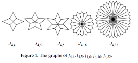
Theorem 2.1. Let \(J_{m,n}\) be the jahangir's graph. Then

  1. \(MZ^{a}_{1}(J_{m,n})=(4)^{am(n-2)}\times (5)^{2am}\times (3+m)^{am}\),
  2. \(MZ^{a}_{2}(J_{m,n})= (4)^{am(n-2)}\times (6)^{2am}\times (3m)^{am}\),
  3. \(G^{a}AII(J_{m,n})=\left(\frac{2\sqrt{6}}{5}\right)^{2am}\times \left(\frac{2\sqrt{3\times m}}{3+m}\right)^{am}\).

Proof. Let \(G\) be the graph of \(J_{m,n}\). It is clear that the total number of vertices in \(J_{m,n}\) are \(8n+2\) and total number of edges are \(10n+1\) The edge set of \(J_{m,n}\) has following three partitions, $$E_{1}=E_{2,2}=\{e=uv\in E(J_{m,n}): d_{u}=2, d_{v}=2\},$$ $$E_{1}=E_{2,3}=\{e=uv\in E(J_{m,n}): d_{u}=2, d_{v}=3\},$$ and $$E_{1}=E_{3,m}=\{e=uv\in E(J_{m,n}): d_{u}=3, d_{v}=m\}.$$ Now, $$\mid E_{1}(J_{m,n})\mid=m(n-2),$$ $$\mid E_{2}(J_{m,n})\mid=2m,$$ and $$\mid E_{1}(J_{m,n})\mid=m.$$

    (1) \begin{eqnarray*} MZ^{a}_{1}(J_{m,n})&=& \prod\limits_{uv\in E(G)}(d_{u}+d_{v})^{a}\\ &=& \prod\limits_{uv\in E_{1}(J_{m,n})}(d_{u}+d_{v})^{a}+\prod\limits_{uv\in E_{2}(J_{m,n})}(d_{u}+d_{v})^{a}+\prod\limits_{uv\in E_{3}(J_{m,n})}(d_{u}+d_{v})^{a}\\ &=&(d_{u}+d_{v})^{a|E_{1}(J_{m,n})|}+(d_{u}+d_{v})^{a|E_{2}(J_{m,n})|}+(d_{u}+d_{v})^{a|E_{3}(J_{m,n})|}\\ &=& (2+2)^{am(n-2)}+(2+3)^{a(2m)}+(3+m)^{am}\\ &=&(4)^{am(n-2)}\times (5)^{2am}\times (3+m)^{am}. \end{eqnarray*} (2) \begin{eqnarray*} MZ^{a}_{2}(J_{m,n})&=& \prod\limits_{uv\in E(G)}(d_{u}.d_{v})^{a}\\ &=& \prod\limits_{uv\in E_{1}(J_{m,n})}(d_{u}.d_{v})^{a}+\prod\limits_{uv\in E_{2}(J_{m,n})}(d_{u}.d_{v})^{a}+\prod\limits_{uv\in E_{3}(J_{m,n})}(d_{u}.d_{v})^{a}\\ &=&(d_{u}.d_{v})^{a|E_{1}(J_{m,n})|}+(d_{u}.d_{v})^{a|E_{2}(J_{m,n})|}+(d_{u}.d_{v})^{a|E_{3}(J_{m,n})|}\\ &=& (2.2)^{am(n-2)}+(2.3)^{a(2m)}+(3.m)^{am}\\ &=&(4)^{am(n-2)}\times (6)^{2am}\times (3m)^{am}. \end{eqnarray*} (3) \begin{eqnarray*} G^{a}AII(J_{m,n})&=& \prod\limits_{uv\in E(G)}\left(\frac{2\sqrt{d_{u}d_{v}}}{d_{u}+d_{v}}\right)^{a}\\ &=& \prod\limits_{uv\in E(G)}\left(\frac{2\sqrt{d_{u}d_{v}}}{d_{u}+d_{v}}\right)^{a}+\prod\limits_{uv\in E(G)}\left(\frac{2\sqrt{d_{u}d_{v}}}{d_{u}+d_{v}}\right)^{a}\\ &&+\prod\limits_{uv\in E(G)}\left(\frac{2\sqrt{d_{u}d_{v}}}{d_{u}+d_{v}}\right)^{a}\\ &=&\left(\frac{2\sqrt{d_{u}d_{v}}}{d_{u}+d_{v}}\right)^{a|E_{1}(J_{m,n})|}\times \left(\frac{2\sqrt{d_{u}d_{v}}}{d_{u}+d_{v}}\right)^{a|E_{2}(J_{m,n})|}\\ &&\times \left(\frac{2\sqrt{d_{u}d_{v}}}{d_{u}+d_{v}}\right)^{a|E_{3}(J_{m,n})|}\\ &=&\left(\frac{2\sqrt{2.2}}{2+2}\right)^{am(n-2)}\times \left(\frac{2\sqrt{2.3}}{2+3}\right)^{a(2m)}\\ &&\times \left(\frac{2\sqrt{3.m}}{3+m}\right)^{am}\\ &=&\left(\frac{2\sqrt{6}}{5}\right)^{2am}\times \left(\frac{2\sqrt{3\times m}}{3+m}\right)^{am}. \end{eqnarray*}

Corollary 2.2. Let \(J_{m,n}\) be the Jahangir's graph. Then

  1. \(MZ_{1}(J_{m,n})=(4)^{m(n-2)}\times (5)^{2m}\times (3+m)^{m}\),
  2. \(MZ_{2}(J_{m,n})= (4)^{m(n-2)}\times (6)^{2m}\times (3m)^{m}\),
  3. \(GAII(J_{m,n})=\left(\frac{2\sqrt{6}}{5}\right)^{2m}\times \left(\frac{2\sqrt{3\times m}}{3+m}\right)^{m}\).

Proof. We get our result by putting \(\alpha=1\) in the Theorem 2.1.

Corollary 2.3. Let \(J_{m,n}\) be the Jahangir's graph. Then

  1. \(H II_{1}(J_{m,n})=(4)^{2m(n-2)}\times (5)^{4m}\times (3+m)^{2m}\),
  2. \(H II_{2}(J_{m,n})= (4)^{2m(n-2)}\times (6)^{4m}\times (3m)^{am}\).

Proof. We get our desired results by putting \(\alpha=2\) in Theorem 2.1.

Corollary 2.4. Let \(J_{m,n}\) be the Jahangir's graph. Then

  1. \(X II(J_{m,n})=\left(\frac{1}{2}\right)^{m(n-2)}\times \left(\frac{1}{\sqrt{5}}\right)^{2m}\times \left(\frac{1}{\sqrt{m+1}}\right)^{mn}\),
  2. \(\chi II(J_{m,n})=\left(\frac{1}{2}\right)^{m(n-2)}\times \left(\frac{1}{\sqrt{6}}\right)^{2m}\times \left(\frac{1}{\sqrt{m+1}}\right)^{mn}\).

Proof. We get our desired results by putting \(\alpha=\frac{-1}{2}\) in Theorem 2.1.

Theorem 2.5. Let \(J_{m,n}\) be the Jahangir's graph. Then $$ABCII(J_{m,n})=\left(\frac{1}{\sqrt{2}}\right)^{mn}\times \left(\sqrt{\frac{m+1}{3m}}\right)^{mn}.$$

Proof. By using the edge partition of Jahangir's graph given in Theorem 2.1. \begin{eqnarray*} ABCII(J_{m,n})&=&\prod\limits_{uv\in E(J_{m,n})}\sqrt{\frac{d_{u}+d_{u}-2}{d_{u}.d_{u}}}\\ &=&\prod\limits_{uv\in E_{1}(J_{m,n})}\sqrt{\frac{d_{u}+d_{u}-2}{d_{u}.d_{u}}}\times \prod\limits_{uv\in E_{2}(J_{m,n})}\sqrt{\frac{d_{u}+d_{u}-2}{d_{u}.d_{u}}}\\ &&\times \prod\limits_{uv\in E_{3}(J_{m,n})}\sqrt{\frac{d_{u}+d_{u}-2}{d_{u}.d_{u}}}\\ &=&\left(\sqrt{\frac{d_{u}+d_{u}-2}{d_{u}.d_{u}}}\right)^{|E_{1}(J_{m,n})|}\times \left(\sqrt{\frac{d_{u}+d_{u}-2}{d_{u}.d_{u}}}\right)^{|E_{2}(J_{m,n})|}\\ &&\times \left(\sqrt{\frac{d_{u}+d_{u}-2}{d_{u}.d_{u}}}\right)^{|E_{3}(J_{m,n})|}\\ &=&\left(\sqrt{\frac{d_{u}+d_{u}-2}{d_{u}.d_{u}}}\right)^{m(n-2)}\times \left(\sqrt{\frac{d_{u}+d_{u}-2}{d_{u}.d_{u}}}\right)^{2m}\\ &&\times \left(\sqrt{\frac{d_{u}+d_{u}-2}{d_{u}.d_{u}}}\right)^{m}\\ &=&\left(\sqrt{\frac{1}{2}}\right)^{m(n-2)}\times \left(\sqrt{\frac{1}{2}}\right)^{2m}\times \left(\sqrt{\frac{m+1}{3m}}\right)^{mn} \\ &=& \left(\frac{1}{\sqrt{2}}\right)^{mn}\times \left(\sqrt{\frac{m+1}{3m}}\right)^{mn} \end{eqnarray*}

Competing Interests

The authors declare that they have no competing interests.

References

  1. Wiener, H. (1947). Structural determination of paraffin boiling points. Journal of the American Chemical Society, 69(1), 17-20. [Google Scholor]
  2. Katritzky, A. R., Jain, R., Lomaka, A., Petrukhin, R., Maran, U., & Karelson, M. (2001). Perspective on the relationship between melting points and chemical structure. Crystal Growth & Design, 1(4), 261-265. [Google Scholor]
  3. Rücker, G., & Rücker, C. (1999). On topological indices, boiling points, and cycloalkanes. Journal of chemical information and computer sciences, 39(5), 788-802. [Google Scholor]
  4. Dobrynin, A. A., Entringer, R., & Gutman, I. (2001). Wiener index of trees: theory and applications. Acta Applicandae Mathematica , 66(3), 211-249. [Google Scholor]
  5. Du, W., Li, X., & Shi, Y. (2009). Algorithms and extremal problem on Wiener polarity index. MATCH Commun. Math. Comput. Chem, 62(1), 235. [Google Scholor]
  6. Gutman, I., & Polansky, O. E. (2012). Mathematical concepts in organic chemistry. Springer Science & Business Media. [Google Scholor]
  7. Ma, J., Shi, Y., & Yue, J. (2014). The Wiener Polarity Index of Graph Products. Ars Comb., 116, 235-244. [Google Scholor]
  8. Ma, J., Shi, Y., Wang, Z., & Yue, J. (2016). On Wiener polarity index of bicyclic networks. Scientific reports, 6, 19066. [Google Scholor]
  9. Gutman, I. (1993). Some properties of the Wiener polynomial. Graph Theory Notes New York , 125, 13-18. [Google Scholor]
  10. Deutsch, E., & Klavžar, S. (2015). M-polynomial and degree-based topological indices. Iran. J. Math. Chem., (6) 93–102. [Google Scholor]
  11. Gutman, I., & Trinajstić, N. (1972). Graph theory and molecular orbitals. Total φ-electron energy of alternant hydrocarbons. Chemical Physics Letters, 17(4), 535-538. [Google Scholor]
  12. Gutman, I., Ruscić, B., Trinajstić, N., & Wilcox Jr, C. F. (1975). Graph theory and molecular orbitals. XII. Acyclic polyenes. The Journal of Chemical Physics, 62(9), 3399-3405. [Google Scholor]
  13. Narumi, H., & Katayama, M. (1984). Simple topological index: A newly devised index characterizing the topological nature of structural isomers of saturated hydrocarbons. Memoirs of the Faculty of Engineering, Hokkaido University, 16(3), 209-214. [Google Scholor]
  14. Gutman, I. (2011). Multiplicative Zagreb indices of trees. Bull. Soc. Math. Banja Luka, 18, 17-23. [Google Scholor]
  15. Todeschini, R., Ballabio, D., & Consonni, V. (2010). Novel molecular descriptors based on functions of new vertex degrees. Mathematical Chemistry Monographs, 73-100. [Google Scholor]
  16. Todeschini, R., & Consonni, V. (2010). New local vertex invariants and molecular descriptors based on functions of the vertex degrees. MATCH Commun. Math. Comput. Chem., 64(2), 359-372. [Google Scholor]
  17. Wang, S., & Wei, B. (2015). Multiplicative Zagreb indices of k-trees. Discrete Applied Mathematics, 180, 168-175. [Google Scholor]
  18. Eliasi, M., Iranmanesh, A., & Gutman, I. (2012). Multiplicative versions of first Zagreb index. MATCH Commun. Math. Comput. Chem., 68(1), 217. [Google Scholor]
  19. Kulli, V. R. (2016). Multiplicative hyper-zagreb indices and coindices of graphs: computing these indices of some nanostructures. International Research Journal of Pure Algebra, 6(7),342-347.[Google Scholor]
  20. Kulli, V. R., Stone, B., Wang, S., & Wei, B. (2017). Generalised multiplicative indices of polycyclic aromatic hydrocarbons and benzenoid systems. Zeitschrift für Naturforschung A, 72(6), 573-576. [Google Scholor]
  21. Kulli, V. R. (2016). Multiplicative connectivity indices of \(TUC_{4}C_{8}[m,n]\) and \(TUC_{4}[m,n]\) nanotubes. Journal of Computer and Mathematical Sciences, 7(11), 599-605. [Google Scholor]