
Chemical graph theory is a branch of graph theory in which a chemical compound is represented by simple graph called molecular graph in which vertices are atoms of compound and edges are the atomic bounds. A graph is connected if there is atleast one connection between its vertices. Throughout this paper we take \(G\) a connected graph. If a graph does not contain any loop or multiple edges then it is called a network. Between two vertices \(u\) and \(v\), the distance is the shortest path between them and is denoted by in graph \(G\). For a vertex \(v\) of \(G\) the degree is number of vertices attached with it. The edge connecting the vertices \(u\) and \(v\) will be denoted by \(uv\). Let \(d_{G}(e)\) denote the degree of an edge \(e\) in \(G\), which is defined by \(d_{G}(e)=d_{G}(u) + d_{G}(v)- 2\) with \(e=uv\). The degree and valence in chemistry are closely related with each other. We refer the book [1] for more details. Now a day another emerging field is Cheminformatics, which helps to predict biological activities with the relationship of Structure-property and quantitative structure-activity. Topological indices and Physico-chemical properties are used in prediction of bioactivity if underlined compounds are used in these studies [2,3 ].
A number that describe the topology of a graph is called topological index. In 1947, the first and most studied topological index was introduced by Weiner [4]. For more details about this index can be found in [5, 6]. In 1975, Milan Randic introduced the Randic index [7]. Bollobas et al. [8] and Amic et al. [9] in 1998, working independently defined the generalized Randic index. This index was studied by both mathematicians and chemists [10]. For details about topological indices, we refer [11,12 ] The first and second \(K\)-Banhatti indices of \(G\) are defined as:
$$B_{1}(G)=\sum\limits_{ue}[d_{G}(u)+d_{G}(e)]$$ and $$B_{2}(G)=\sum\limits_{ue}[d_{G}(u)\times d_{G}(e)]$$ where ue means that the vertex \(u\) and edge e are incident in \(G\). The first and second K-hyper Banhatti indices of G are defined as $$HB_{1}(G)=\sum\limits_{ue}[d_{G}(u)+d_{G}(e)]^{2}$$ and $$HB_{2}(G)=\sum\limits_{ue}[d_{G}(u)\times d_{G}(e)]^{2}.$$ We refer [13] for details about these indices. The David derived and dominating David derived network of dimension \(n\) can be constructed as follows [14]: consider a n dimensional star of David network . Insert a new vertex on each edge and split it into two parts, we will get David derived network \(DD(n)\) of dimension \(n\).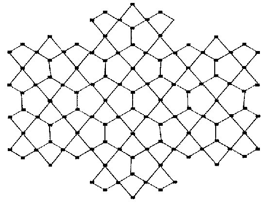
Theorem 1.1 Let \(G=D_{1}(n)\) be the dominating David derived network of \(1^{st}\) type. Then the first and the second \(K\)-Banhatti indices of \(D_{1}(n)\) are \begin{eqnarray*} B_{1}[D_{1}(n)]&=&1485n^{2}+1624n-1002\\ B_{2}[D_{1}(n)]&=&3204n^{2}+764n-3292 \end{eqnarray*}
Proof. Let \(G=D_{1}(n)\) be the dominating David derived network of \(1^{st}\) type. From figure 1, the edge partition of dominating David derived network of \(1^{st}\) type \(D_{1}(n)\) based on degrees of end vertices of each edge is give in table 1.
| \((d_{u}, d_{v})\) | Number of edges | Degree of Edges |
|---|---|---|
| \((2,2)\) | \(4n\) | \(2\) |
| \((2,3)\) | \(4n-4\) | \(3\) |
| \((2,4)\) | \(28n-16\) | \(4\) |
| \((3,3)\) | \(9n^{2}-13n+24\) | \(4\) |
| \((3,4)\) | \(36n^{2}-56n+24\) | \(5\) |
| \((4,4)\) | \(36n^{2}-56n+20\) | \(6\) |
Theorem 1.2. Let \(G=D_{1}(n)\) be the dominating David derived network of \(1^{st}\) type. Then the first and the second \(K\)-hyper Banhatti indices of \(D_{1}(n)\) are \begin{eqnarray*} HB_{1}[D_{1}(n)]&=&13302n^{2}-16623n+6146\\ HB_{2}[D_{1}(n)]&=&66564n^{2}-89092n+33892 \end{eqnarray*}
Proof Let \(G=D_{1}(n)\) be the dominating David derived network of \(1^{st}\) type. Then first \(K\)-hyper Banhatti index of \(D_{1}(n)\) is calculated as \begin{eqnarray*} HB_{1}[D_{1}(n)]&=&\sum\limits_{ue}[d_{G}(u)+d_{G}(v)]^{2}\\ &=&\sum\limits_{ue\in E_{2,2}}[(d_{G}(u)+d_{G}(e))^{2}+(d_{G}(v)+d_{G}(e))^{2}]\\ &&+ \sum\limits_{ue\in E_{2,3}}[(d_{G}(u)+d_{G}(e))^{2}+(d_{G}(v)+d_{G}(e))^{2}]\\ &&+\sum\limits_{ue\in E_{2,4}}[(d_{G}(u)+d_{G}(e))^{2}+(d_{G}(v)+d_{G}(e))^{2}]\\ &&+\sum\limits_{ue\in E_{3,3}}[(d_{G}(u)+d_{G}(e))^{2}+(d_{G}(v)+d_{G}(e))^{2}]\\ &&+\sum\limits_{ue\in E_{3,4}}[(d_{G}(u)+d_{G}(e))^{2}+(d_{G}(v)+d_{G}(e))^{2}]\\ &&+\sum\limits_{ue\in E_{4,4}}[(d_{G}(u)+d_{G}(e))^{2}+(d_{G}(v)+d_{G}(e))^{2}]\\ &=& 4n[(2+2)^{2}+(2+2)^{2}]+(4n-4)[(2+3)^{2}+(3+3)^{2}]\\ &&+(28n-16)[(2+4)^{2}+(4+4)^{2}]\\ &&+(9n^{2}-13n+24)[(3+4)^{2}+(3+4)^{2}]\\ &&+(36n^{2}-56n+24)[(3+5)^{2}+(4+5)^{2}]\\ &&+(36n^{2}-56n+20)[(4+6)^{2}+(4+6)^{2}]\\ &=& 13302n^{2}-16623n+6146 \end{eqnarray*} Second \(K\)-hyper Banhatti index of \(D_{1}(n)\) is calculated as \begin{eqnarray*} HB_{2}[D_{1}(n)]&=&\sum\limits_{ue}[d_{G}(u)d_{G}(v)]^{2}\\ &=&\sum\limits_{ue\in E_{2,2}}[(d_{G}(u)d_{G}(e))^{2}+(d_{G}(v)d_{G}(e))^{2}]\\ &&+ \sum\limits_{ue\in E_{2,3}}[(d_{G}(u)d_{G}(e))^{2}+(d_{G}(v)d_{G}(e))^{2}]\\ &&+\sum\limits_{ue\in E_{2,4}}[(d_{G}(u)d_{G}(e))^{2}+(d_{G}(v)d_{G}(e))^{2}]\\ &&+\sum\limits_{ue\in E_{3,3}}[(d_{G}(u)d_{G}(e))^{2}+(d_{G}(v)d_{G}(e))^{2}]\\ &&+\sum\limits_{ue\in E_{3,4}}[(d_{G}(u)d_{G}(e))^{2}+(d_{G}(v)d_{G}(e))^{2}]\\ &&+\sum\limits_{ue\in E_{4,4}}[(d_{G}(u)d_{G}(e))^{2}+(d_{G}(v)d_{G}(e))^{2}]\\ &=& 4n[4^{2}+4^{2}]+(4n-4)[6^{2}+9^{2}]\\ &&+(28n-16)[8^{2}+16^{2}]\\ &&+(9n^{2}-13n+24)[12^{2}+12^{2}]\\ &&+(36n^{2}-56n+24)[15^{2}+20^{2}]\\ &&+(36n^{2}-56n+20)[24^{2}+24^{2}]\\ &=& 66564n^{2}-89092n+33892. \end{eqnarray*}
Theorem 1.3. Let \(G=D_{2}(n)\) be the dominating David derived network of \(2^{nd}\) type. Then the first and the second \(K\)-Banhatti indices of \(D_{2}(n)\) are \begin{eqnarray*} B_{1}[D_{2}(n)]&=&1530n^{2}-1810n+650\\ B_{2}[D_{2}(n)]&=&32584n^{2}-4127n+1506 \end{eqnarray*}
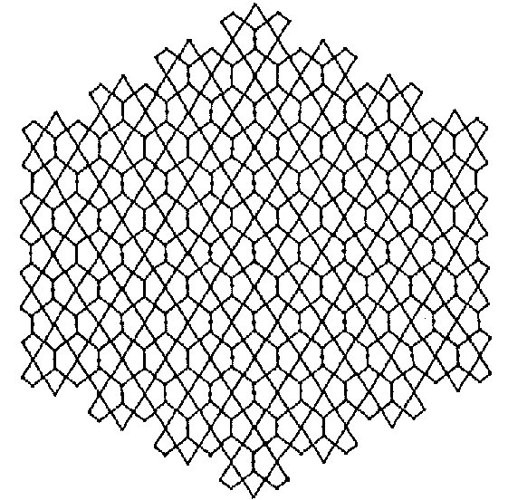
Proof Let \(G=D_{2}(n)\) be the dominating David derived network of \(2^{nd}\) type. Table \(2\) shows the edge partition of dominating David derived network of \(2^{nd}\) type \(D_{2}(n)\) based on degrees of end vertices of each edge
| \((d_{u}, d_{v})\) | Number of edges | Degree of Edges |
|---|---|---|
| \((2,2)\) | \(4n\) | \(2\) |
| \((2,3)\) | \(18n^{2}-22n+6\) | \(3\) |
| \((2,4)\) | \(28n-16\) | \(4\) |
| \((3,4)\) | \(36n^{6}-56n+24\) | \(5\) |
| \((4,4)\) | \(336n^{6}-56n+20\) | \(6\) |
Theorem 1.4. Let \(G=D_{2}(n)\) be the dominating David derived network of \(2^{nd}\) type. Then the first and the second \(K\)-hyper Banhatti indices of \(D_{2}(n)\) are \begin{eqnarray*} HB_{1}[D_{1}(n)]&=&1351n^{2}-1693n+6246\\ HB_{2}[D_{1}(n)]&=&22606n^{2}-28486n+10582 \end{eqnarray*}
Proof Let \(G=D_{2}(n)\) be the dominating David derived network of \(2^{nd}\) type. First \(K\)- hyper Banhatti index of \(D_{2}(n)\) is calculated as \begin{eqnarray*} HB_{1}[D_{2}(n)]&=&\sum\limits_{ue}[d_{G}(u)+d_{G}(v)]^{2}\\ &=&\sum\limits_{ue\in E_{2,2}}[(d_{G}(u)+d_{G}(e))^{2}+(d_{G}(v)+d_{G}(e))^{2}]\\ &&+ \sum\limits_{ue\in E_{2,3}}[(d_{G}(u)+d_{G}(e))^{2}+(d_{G}(v)+d_{G}(e))^{2}]\\ &&+\sum\limits_{ue\in E_{2,4}}[(d_{G}(u)+d_{G}(e))^{2}+(d_{G}(v)+d_{G}(e))^{2}]\\ &&+\sum\limits_{ue\in E_{3,4}}[(d_{G}(u)+d_{G}(e))^{2}+(d_{G}(v)+d_{G}(e))^{2}]\\ &&+\sum\limits_{ue\in E_{4,4}}[(d_{G}(u)+d_{G}(e))^{2}+(d_{G}(v)+d_{G}(e))^{2}]\\ &=& 4n[(2+2)^{2}+(2+2)^{2}]+(18n^{2}-22n+6)[(2+3)^{2}+(3+3)^{2}]\\ &&+(28n-16)[(2+4)^{2}+(4+4)^{2}]\\ &&+(36n^{6}-56n+24)[(3+5)^{2}+(4+5)^{2}]\\ &&+(36n^{6}-56n+20)[(4+6)^{2}+(4+6)^{2}]\\ &=& 1351n^{2}-1693n+6246. \end{eqnarray*} Second \(K\)-hyper Banhatti index of \(D_{2}(n)\) is calculated as \begin{eqnarray*} HB_{2}[D_{2}(n)]&=&\sum\limits_{ue}[d_{G}(u)d_{G}(v)]^{2}\\ &=&\sum\limits_{ue\in E_{2,2}}[(d_{G}(u)d_{G}(e))^{2}+(d_{G}(v)d_{G}(e))^{2}]\\ &&+ \sum\limits_{ue\in E_{2,3}}[(d_{G}(u)d_{G}(e))^{2}+(d_{G}(v)d_{G}(e))^{2}]\\ &&+\sum\limits_{ue\in E_{2,4}}[(d_{G}(u)d_{G}(e))^{2}+(d_{G}(v)d_{G}(e))^{2}]\\ &&+\sum\limits_{ue\in E_{3,4}}[(d_{G}(u)d_{G}(e))^{2}+(d_{G}(v)d_{G}(e))^{2}]\\ &&+\sum\limits_{ue\in E_{4,4}}[(d_{G}(u)d_{G}(e)^{2})+(d_{G}(v)d_{G}(e))^{2}]\\ &=& 4n[(2.2)^{2}+(2.2)^{2}]+(18n^{2}-22n+6)[(2.3)^{2}+(3.3)^{2}]\\ &&+(28n-16)[(2.4)^{2}+(4.4)^{2}]\\ &&+(36n^{6}-56n+24)[(3.5)^{2}+(4.5)^{2}]\\ &&+(36n^{6}-56n+20)[(4.6)^{2}+(4.6)^{2}]\\ &=& 22606n^{2}-28486n+10582. \end{eqnarray*}
Theorem 1.5 Let \(G=D_{3}(n)\) be the dominating David derived network of \(3^{rd}\) type. Then the first and the second $K$-Banhatti indices of \(D_{3}(n)\) are \begin{eqnarray*} B_{1}[D_{3}(n)]&=&1944n^{2}-2128n+600\\ B_{2}[D_{3}(n)]&=&4320n^{2}-8224n+2112 \end{eqnarray*}
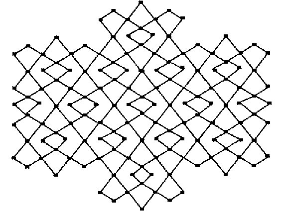
Proof Let \(G=D_{3}(n)\) be the dominating David derived network of \(3^{rd}\) type. Table \(3\) shows the edge partition of dominating David derived network of \(3^{rd}\) type \(D_{3}(n)\) based on degrees of end vertices of each edge.
| \((d_{u}, d_{v})\) | Number of edges | Degree of Edges |
|---|---|---|
| \((2,2)\) | \(4n\) | \(2\) |
| \((2,4)\) | \(36n^{2}-20n\) | \(4\) |
| \((4,4)\) | \(72n^{2}-108n+44\) | \(6\) |
Theorem 1.6. Let \(G=D_{3}(n)\) be the dominating David derived network of \(3^{rd}\) type. Then the first and the second \(K\)-hyper Banhatti indices of \(D_{3}(n)\) are \begin{eqnarray*} HB_{1}[D_{3}(n)]&=&18000n^{2}-23472n+8800\\ HB_{2}[D_{3}(n)]&=&94464n^{2}-130688n+50688 \end{eqnarray*}
Proof. Let \(G=D_{3}(n)\) be the dominating David derived network of \(3^{rd}\) type. Then the first \(K\)-hyper Banhatti index is calculated as \begin{eqnarray*} HB_{1}[D_{3}(n)]&=&\sum\limits_{ue}[d_{G}(u)+d_{G}(v)]^{2}\\ &=&\sum\limits_{ue\in E_{2,2}}[(d_{G}(u)+d_{G}(e))^{2}+(d_{G}(v)+d_{G}(e))^{2}]\\ &&+ \sum\limits_{ue\in E_{2,4}}[(d_{G}(u)+d_{G}(e))^{2}+(d_{G}(v)+d_{G}(e))^{2}]\\ &&+\sum\limits_{ue\in E_{4,4}}[(d_{G}(u)+d_{G}(e))^{2}+(d_{G}(v)+d_{G}(e))^{2}]\\ &=& 4n[(2+2)^{2}+(2+2)^{2}]+(36n^{2}-20n)[(2+4)^{2}+(4+4)^{2}]\\ &&+(72n^{2}-108n+44)[(2+6)^{2}+(4+6)^{2}]\\ &=& 18000n^{2}-23472n+8800 \end{eqnarray*} Second \(K\)-hyper Banhatti index of \(D_{3}(n)\) is calculated as \begin{eqnarray*} HB_{1}[D_{3}(n)]&=&\sum\limits_{ue}[d_{G}(u)+d_{G}(v)]^{2}\\ &=&\sum\limits_{ue\in E_{2,2}}[(d_{G}(u)d_{G}(e))^{2}+(d_{G}(v)d_{G}(e))^{2}]\\ &&+ \sum\limits_{ue\in E_{2,4}}[(d_{G}(u)d_{G}(e))^{2}+(d_{G}(v)d_{G}(e))^{2}]\\ &&+\sum\limits_{ue\in E_{4,4}}[(d_{G}(u)d_{G}(e))^{2}+(d_{G}(v)d_{G}(e))^{2}]\\ &=& 4n[(2.2)^{2}+(2.2)^{2}]+(36n^{2}-20n)[(2.4)^{2}+(4.4)^{2}]\\ &&+(72n^{2}-108n+44)[(2.6)^{2}+(4.6)^{2}]\\ &=& 94464n^{2}-130688n+50688 \end{eqnarray*}