Chemical reaction network theory is an area of applied mathematics that attempts to model the behavior of real world chemical systems. Since its foundation in the 1960s, it has attracted a growing research community, mainly due to its applications in biochemistry and theoretical chemistry. It has also attracted interest from pure mathematicians due to the interesting problems that arise from the mathematical structures involved. In this report, we compute newly defined topological indices, namely, Arithmetic-Geometric index (\(AG_{1}\) index), \(SK\) index, \(SK_{1}\) index, and \(SK_{2}\) index of the Honey Comb Derived Networks. We also compute sum connectivity index and modified Randić index. Moreover we give geometric comparison of our results.
A topological index is a numeric quantity, which is invariant up to graph isomorphism, associated with the chemical constitution of a chemical compound aiming the correlation of chemical structure with many of its physico-chemical properties, chemical reactivity or biological activities. Topological indices are designed on the ground of transformation of a molecular graph into a number which characterize the topology of that graph.
For example, a fixed interconnection parallel architecture is characterized by a graph, with vertices corresponding to processing edges and nodes representing communication links. In hard to compare Interconnection networks are notoriously in abstract terms. Thus, in parallel processing, researchers are motivated to propose improved interconnection networks, offering performance evaluations and arguing the benefits in different contexts [1, 2, 3]. A few networks such as grid, honeycomb and hexagonal networks, for instance, bear resemblance to molecular or atomic lattice structures. These networks have interesting topological properties which have been studied in [4, 5, 6, 7, 8].
The honeycomb and hexagonal networks have been known as crucial for evolutionary biology, in particular for the evolution of cooperation, where the overlapping triangles are vital for the propagation of cooperation in social dilemmas. For relevant research, see [9, 10].
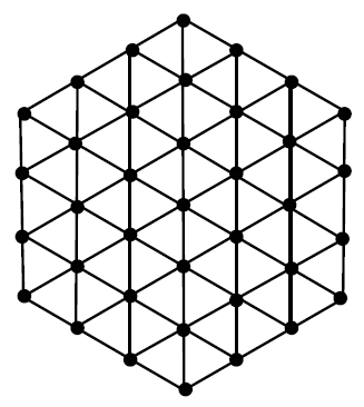
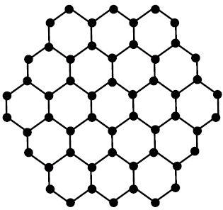
In hexagonal network \(HX(n)\) the parameter \(n\) is the number of vertices on each side of the network see figure 1, whereas for honeycomb network \(HC(n)\),\(n\) is the number of hexagons between boundary and central hexagon see figure 2. Due to significance of topological indices in chemistry, a lot of research has been done in this area. For further studies of topological indices of various graph families, see [11, 12, 13, 14, 15].
Figure 1. Hexagonal network.Figure 2. Honeycomb network.
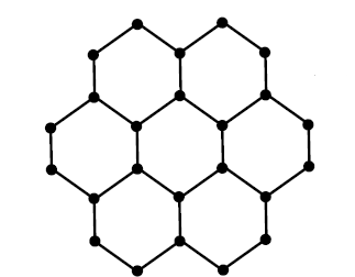
Let us consider a graph as shown in figure 3
Figure 3. Graph \(G\).
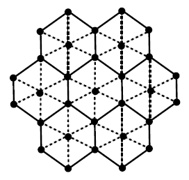
The stellation of \(G\) is denoted by \(St(G)\) and can be obtained by adding a vertex in each face of $G$ and then by join these vertices to all vertices of the respective face (see figure 4).
Figure 4. Stellation of \(G\) (dotted).
The dual \(Du(G)\) of a graph \(G\) is a graph that has a vertex for each face of \(G\). The graph has an edge whenever two faces of \(G\) are separated from each other, and a self-loop when the same face appears on both sides of an edge, see Figure 5. Hence the number of faces of a graph is equal to the number of edges of its dual.
Figure 5. Dual of graph \(G\) (dotted).
In dual graph, if we delete the vertex corresponding to the bounded face of planer graph, which is unique in it, we get bounded dual \(Bdu(G)\) (see Figure 6).
Figure 6. Bounded dual of graph \(G\) (dotted).
Given a connected plane graph \(G\), its medial graph \(M(G)\) has a vertex for each edge of \(G\) and an edge between two vertices for each face of \(G\) in which their corresponding edges occur consecutively (see Figure 7).
Figure 7. Medial of \(G\) (dotted).
In this report, we aim to compute degree-based topological indices of networks derived from honeycomb networks by taking Stellation, dual and bounded dual and Medial of honeycomb network.
2. Basic definitions and background of problem
A molecular graph is a simple graph in chemical graph theory, in which atoms are represented by vertices and chemical bonds are represented by edges. A graph is connected if there is a connection between any pair of vertices. A network is a connected graph which has no multiple edge and loop. The number of vertices which are connected to a fixed \(v\) vertex is called the degree of \(v\) and is denoted by \(d_{v}\). The distance between two vertices is the length of shortest path between them. The concept of valence in chemistry and concept of degree is somewhat closely. For details on bases of graph theory, we refer the book [16]. Quantitative structure-activity and Structure-property relationships predict the properties and biological activities of unstudied material. In these studies, topological indices and some Physico-chemical properties are used to predict bioactivity of the chemical compounds [17, 18, 19, 20]. A topological index of the graph of a chemical compound is a number, which can be used to characterize the underlined chemical compound and help to predict its physiochemical properties. Weiner laid the foundation of Topological index in 1947. He was approximated the boiling point of alkanes and introduced the Weiner index [21]. The Weiner index is defined as
\begin{equation*}
W(G)=\frac{1}{2}\sum\limits_{uv}d(u,v).
\end{equation*}
Till now more than 140 topological indices are defined but no single index is enough to determine all physico-chemical properties, but, these topological indices together can do this to some extent. Later, in 1975, Milan Randić introduced Randić index, [22].
\begin{equation*}
R_{\frac{-1}{2}}=\sum\limits_{uv\in E(G)}\frac{1}{\sqrt{d_{u}d_{v}}}.
\end{equation*}
In 1998, Bollobas and Erdos [23] and Amic et al. [24] proposed the generalized Randić index and has been studied by both chemist and mathematicians [25].
\begin{equation*}
R_{\alpha}(G)=\sum\limits_{uv\in E(G)}(d_{u}d_{v})^{\alpha}.
\end{equation*}
The Randić index is one of the most popular and most studied and applied topological index. Many reviews, papers and books [26, 27, 28, 29, 30, 31] are written on this simple graph invariant
The first Zagreb index and second Zagreb index was introduced by Gutman and Trinajstić as
\begin{equation*}
M_{1}(G)=\sum\limits_{uv\in E(G)}(d_{u}+d_{v}),
\end{equation*}
\begin{equation*}
M_{2}(G)=\sum\limits_{uv\in E(G)}(d_{u}d_{v})
\end{equation*}
respectively. See [ 32, 33, 34, 35, 36 ] for detail. Sum connectivity index is defined as
\begin{equation*}
\chi(G)=\sum\limits_{uv\in E(G)}\frac{1}{\sqrt{d_{u}+d_{v}}}
\end{equation*}
and modified Randić index is defined as
\begin{equation*}
R'(G)=\sum\limits_{uv\in E(G)}\frac{1}{\max\{d_{u},d_{v}\}}.
\end{equation*}
V. S. Shigehalli and Rachanna Kanabur [ 37] introduced following new degree-based topological indices:
\begin{equation*}
AG_{1}=\sum\limits_{uv\in E(G)}\frac{1}{2\sqrt{d_{u}+d_{v}}},\;\;
SK=\sum\limits_{uv\in E(G)}\frac{d_{u}+d_{v}}{2},
\end{equation*}
\begin{equation*}
SK_{1}=\sum\limits_{uv\in E(G)}\frac{d_{u}d_{v}}{2},
\end{equation*}
\begin{equation*}
SK_{2}=\sum\limits_{uv\in E(G)}\left(\frac{d_{u}+d_{v}}{2}\right)^{2}.
\end{equation*}
3. Main Results
In this section we present our computational results.
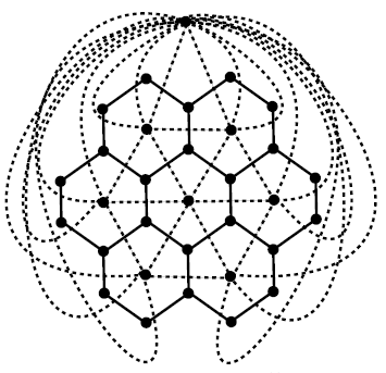
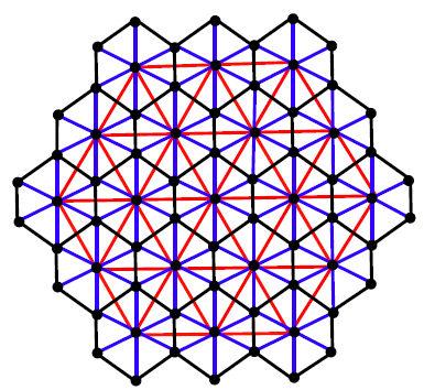
Honey Comb derived network of dimension 1 is obtained by taking the union of honey comb network and its stellation (see Figure 8), which is a planar graph.
In this section, we will present our computational results
Theorem 3.1.
Let \(HcDN1(n)\) be the Honey Comb Derived Network of dimension 1. Then
Proof.
Let \(HcDN1(n)\) be the Honey Comb Derived Network of dimension 1 shown in figure 8.
Figure 8. \(HcDN1(n)\) network with \(n=3\).
The number of vertices and edges in \(HcDN1(n)\) are \(9n^{2}-3n+1\) and \(27n^{2}-3n+1\) respectively. There are five types of edges in \(HcDN1(n)\) based on degrees of end vertices of each edge. Table 1 shows such an edge partition of \(HcDN1(n)\).
Proof.
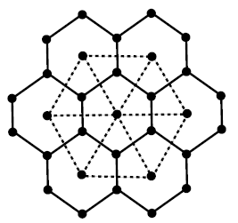
Let \(HcDN2(n)\) be honey Comb Derived Network of dimension 2 shown in figure 9. The number of vertices and edges in \(HcDN2(n)\) are \(9n^{2}-3n+1\) and \(27n^{2}-21n+6\) respectively. There are sixteen types of edges in \(HcDN2(n)\) based on degrees of end vertices of each edge. Table 2 shows such an edge partition of \(HcDN2(n)\).
Figure 9. \(HcDN2(n)\) network with \(n=3\).
Table 2. Edge partition \(HcDN2(n)\)
\((d_{u}, d_{v})\)
Number of edges
\((3,3)\)
\(6\)
\((3,5)\)
\(12(n-1)\)
\((3,9) \)
\(12\)
\((3,10) \)
\(6(n-1)\)
\((3,10) \)
\(6(n-1)\)
\((5,6) \)
\(6(n-2)\)
\((5,9) \)
\(12\)
\((5,10)\)
\(12(n-2)\)
\((6,6) \)
\(9n^{2}-21n+12\)
\((6,9)\)
\(12\)
\((6,10) \)
\(8(n-2)\)
\((6,12) \)
\(18n^{2}-54n+42\)
\((9,10) \)
\(12\)
\((9,12) \)
\(6\)
\((10,10)\)
\(6(n-3)\)
\((10,12)\)
\(12(n-2)\)
\((12,12) \)
\(9n^{2}-33n+30\)
Now, using the edge partition given in Table 2 in the formulas of \(\chi(G)\), \(R'(G)\), \(AG_{1}(G)\), \(SK(G)\), \(SK_{1}(G)\) and \(SK_{2}(G)\) in the similar fashion as in Theorem 3.1, we can get the desired results.
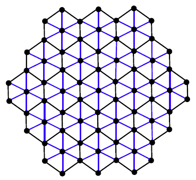
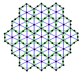
Honey Comb derived network of dimension 3 \(HcDN3(n)\) is obtained by taking the union of honey comb network, its stellation and medial (see Figure 10), which is a non-planar graph.
Theorem 3.3.
Let \(HcDN2(n)\) be the Honey Comb Derived Network of dimension 3. Then
Proof. Let \(HcDN3(n)\) be honey Comb Derived Network of dimension 3 shown in figure 10. The number of vertices and edges in \(HcDN3(n)\) are \(18n^{2}-6n+1\) and \(54n^{2}-42n+12\) respectively. There are seven types of edges in \(HcDN3(n)\) based on degrees of end vertices of each edge. Table 3 shows such an edge partition of \(HcDN3(n)\).
Figure 10. \(HcDN3(n)\) network with \(n=3\).
Table 3. Edge partition \(HcDN3(n)\)
\((d_{u}, d_{v})\)
Number of edges
\((3,4)\)
\(12n\)
\((3,6)\)
\(6n\)
\((4,4)\)
\(6n\)
\((4,5)\)
\(12(n-1)\)
\((4,6)\)
\(12(n-1)\)
\((5,6)\)
\(18(n-1)\)
\((6,6)\)
\(54n^{2}-108n+54\)
Now, using the edge partition given in Table 3 in the formulas of \(\chi(G)\), \(R'(G)\), \(AG_{1}(G)\), \(SK(G)\), \(SK_{1}(G)\) and \(SK_{2}(G)\) in the similar fashion as in Theorem 3.1, we can get the desired results.
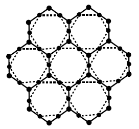
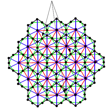
Honey Comb derived network of dimension 4 \(HcDN4(n)\) is obtained by taking the union of honey comb network, its stellation, bounded dual and medial (see Figure 11), which is a non-planar graph.
Theorem 3.4.
Let \(HcDN4(n)\) be the Honey Comb Derived Network of dimension 4. Then
Proof.
Let \(HcDN4(n)\) be honey Comb Derived Network of dimension 4 shown in figure 11. The number of vertices and edges in \(HcDN4(n)\) are \(18n^{2}-6n+1\) and \(63n^{2}-57n+18\) respectively. There are eighteen types of edges in \(HcDN4(n)\) based on degrees of end vertices of each edge. Table 4 shows such an edge partition of \(HcDN4(n)\).
Figure 11. \(HcDN3(n)\) network with \(n=3\).
Table 4. Edge partition \(HcDN4(n)\)
\((d_{u}, d_{v})\)
Number of edges
\((3,4)\)
\(12n\)
\((3,9)\)
\(12\)
\((3,10)\)
\(6(n-2)\)
\((4,4)\)
\(6n\)
\((4,5)\)
\(12(n-1)\)
\((4,6)\)
\(12(n-1)\)
\((5,6)\)
\(6(n-1)\)
\((5,9)\)
\(12\)
\((5,10)\)
\(12(n-3)\)
\((6,6)\)
\(36n^{2}-72n+36\)
\((6,9)\)
\(12\)
\((6,10)\)
\(18(n-2)\)
\((6,12)\)
\(18n^{2}-54n+42\)
\((9,10)\)
\(12\)
\((9,12)\)
\(6\)
\((10,10)\)
\(6(n-3)\)
\((10,12)\)
\(12(n-2)\)
\((12,12)\)
\(9n^{2}-33n+30\)
Now, using the edge partition given in Table 4 in the formulas of \(\chi(G)\), \(R'(G)\), \(AG_{1}(G)\), \(SK(G)\), \(SK_{1}(G)\) and \(SK_{2}(G)\) in the similar fashion as in Theorem 3.1, we can get the desired results.
4. Concluding Remarks and Graphical Comparison
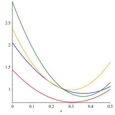
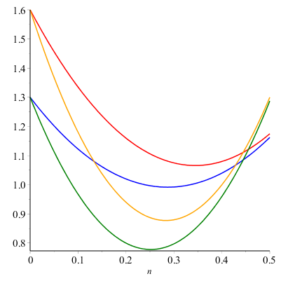
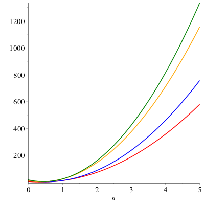
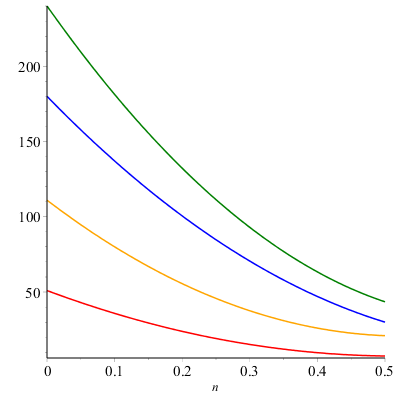
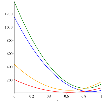
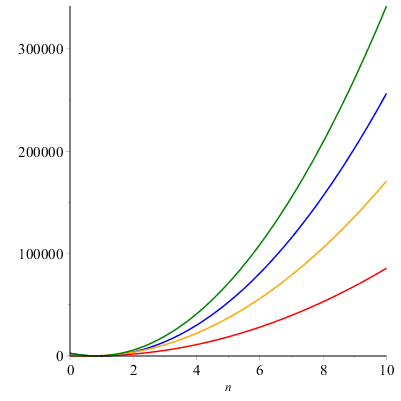
Here we give geometric comparison of results. In figure 12-17 , red, blue, orange and green colors are for honeycomb derived networks of dimension 1, 2, 3 and 4 respectively. With the help of these figures one can choose a network having maximum value and minimums value of topological index. For example from figure 12 it can be observed easily that Honeycomb derived network of dimension 3 has maximum value of sum connectivity index, while honeycomb derived network of dimension 1II has minimum value of sum connectivity index. The figure 13 tells us that Honeycomb derived network of dimension I gives maximum value of modify Randic index and honeycomb derived network of dimension II has minimum value of modify Randic index.
Figure 12. Sum Connectivity Index.Figure 13. Modify Randic Index.Figure 14. AG1 index.Figure 15. SK Index.Figure 16. SK1 Index.Figure 17. SK2 Index.
In this paper we computed some newly defined degree-based topological indices of networks derived from Honey comb networks. Topological indices help us to guess properties of understudy chemical networks.
For example, it has been experimentally verified that the first Zagreb index is directly related with total ? -electron energy. Also Randic index is useful for determining physio-chemical properties of alkanes as noticed by chemist Melan Randic in 1975. He noticed the correlation between the Randic index R and several physico-chemical properties of alkanes like, enthalpies of formation, boiling points, chromatographic retention times, vapor pressure and surface areas. Our next target is to study mathematical properties of understudy topological indices and correlate these indices with chemical properties of networks. To find the bonds of these topological indices for special families of graphs like trees, hyper cubes, bipartite graphs, completer graphs etc is an interesting problems for the researchers working in this direction. Another open problem is to compute distance based topological indices of these networks.
Competing Interests
The authors declare that they have no competing interests.
References
Wang, Z., Szolnoki, A., & Perc, M. (2012). If players are sparse social dilemmas are too: Importance of percolation for evolution of cooperation. Scientific reports , 2, 369. [Google Scholor]
Perc, M., & Szolnoki, A. (2010). Coevolutionary games—a mini review. BioSystems, 99(2), 109-125.[Google Scholor]
Szolnoki, A., Perc, M., & Szabó, G. (2009). Topology-independent impact of noise on cooperation in spatial public goods games. Physical Review E, 80(5), 056109.[Google Scholor]
Bača, M., Horváthová, J., Mokrišová, M., & Suhányiová, A. (2015). On topological indices of fullerenes. Applied Mathematics and Computation, 251, 154-161.[Google Scholor]
Baig, A. Q., Imran, M., & Ali, H. (2015). On topological indices of poly oxide, poly silicate, DOX, and DSL networks. Canadian Journal of chemistry, 93(7), 730-739. [Google Scholor]
Hayat, S., & Imran, M. (2014). Computation of topological indices of certain networks. Applied Mathematics and Computation, 240, 213-228. [Google Scholor]
Imran, M., Hayat, S., & Mailk, M. Y. H. (2014). On topological indices of certain interconnection networks. Applied Mathematics and Computation , 244, 936-951.[Google Scholor]
Xu, J. (2013). Topological structure and analysis of interconnection networks (Vol. 7). Springer Science & Business Media. [Google Scholor]
Imran, M., Baig, A. Q., Ali, H., & Rehman, S. U. (2016). On topological properties of poly honeycomb networks. Periodica Mathematica Hungarica , 73(1), 100-119. [Google Scholor]
Hayat, S., Malik, M. A., & Imran, M. (2015). Computing topological indices of honey-comb derived networks. Romanian journal of Information science and technology, 18, 144-165. [Google Scholor]
Abdo, H., Dimitrov, D., & Gao, W. (2016). On the irregularity of some molecular structures. Canadian Journal of Chemistry, 95(2), 174-183. [Google Scholor]
Ahmadi, M. B., Dimitrov, D., Gutman, I., & Hosseini, S. A. (2014). Disproving a conjecture on trees with minimal atom-bond connectivity index. MATCH Commun. Math. Comput. Chem, 72(3), 685-698. [Google Scholor]
Dimitrov, D. (2016). On structural properties of trees with minimal atom-bond connectivity index II: Bounds on B1-and B2-branches. Discrete Applied Mathematics, 204, 90-116.[Google Scholor]
Dimitrov, D., Du, Z., & da Fonseca, C. M. (2016). On structural properties of trees with minimal atom-bond connectivity index III: Trees with pendent paths of length three. Applied Mathematics and Computation , 282, 276-290.[Google Scholor]
Guirao, J. L. G., & de Bustos, M. T. (2012). Dynamics of pseudo-radioactive chemical products via sampling theory. Journal of Mathematical Chemistry, 50(2), 374-378.[Google Scholor]
West, D. B. (2001). Introduction to graph theory (Vol. 2). Upper Saddle River: Prentice hall.[Google Scholor]
Rücker, G., & Rücker, C. (1999). On topological indices, boiling points, and cycloalkanes. Journal of chemical information and computer sciences, 39(5), 788-802.[Google Scholor]
Klavžar, S., & Gutman, I. (1996). A comparison of the Schultz molecular topological index with the Wiener index. Journal of chemical information and computer sciences, 36(5), 1001-1003.[Google Scholor]
Brückler, F. M., Došlić, T., Graovac, A., & Gutman, I. (2011). On a class of distance-based molecular structure descriptors. Chemical physics letters, 503(4-6), 336-338. [Google Scholor]
Deng, H., Yang, J., & Xia, F. (2011). A general modeling of some vertex-degree based topological indices in benzenoid systems and phenylenes. Computers & Mathematics with Applications, 61(10), 3017-3023. [Google Scholor]
Wiener, H. (1947). Structural determination of paraffin boiling points. Journal of the American Chemical Society, 69(1), 17-20. [Google Scholor]
Randic, M. (1975). Characterization of molecular branching. Journal of the American Chemical Society, 97(23), 6609-6615. [Google Scholor]
Bollobás, B., & Erdös, P. (1998). Graphs of extremal weights. Ars Combinatoria , 50, 225-233. [Google Scholor]
Amić, D., Bešlo, D., Lučić, B., Nikolić, S., & Trinajstić, N. (1998). The vertex-connectivity index revisited. Journal of chemical information and computer sciences, 38(5), 819-822.[Google Scholor]
Hu, Y., Li, X., Shi, Y., Xu, T., & Gutman, I. (2005). On molecular graphs with smallest and greatest zeroth-order general Randic index. MATCH Commun. Math. Comput. Chem, 54(2), 425-434. [Google Scholor]
Li, X., Gutman, I., & Randić, M. (2006). Mathematical aspects of Randić-type molecular structure descriptors. University, Faculty of Science. [Google Scholor]
Randić, M. (2008). On history of the Randić index and emerging hostility toward chemical graph theory. MATCH Commun. Math. Comput. Chem, 59, 5-124. [Google Scholor]
Randić, M. (2001). The connectivity index 25 years after. Journal of Molecular Graphics and Modelling, 20(1), 19-35. [Google Scholor]
Gutman, I., & Furtula, B. (Eds.). (2008). Recent results in the theory of Randić index. University, Faculty of Science. [Google Scholor]
Li, X., & Shi, Y. (2008). A survey on the Randic index. MATCH Commun. Math. Comput. Chem, 59(1), 127-156. [Google Scholor]
Nikolić, S., Kovačević, G., Miličević, A., & Trinajstić, N. (2003). The Zagreb indices 30 years after. Croatica chemica acta, 76(2), 113-124. [Google Scholor]
Gutman, I., & Das, K. C. (2004). The first Zagreb index 30 years after. MATCH Commun. Math. Comput. Chem, 50(1), 83-92. [Google Scholor]
Das, K. C., & Gutman, I. (2004). Some properties of the second Zagreb index. MATCH Commun. Math. Comput. Chem, 52(1), 3-1. [Google Scholor]
Gutman, I., Miličević, A., Nikolić, S., & Trinajstić, N. (2010). About the Zagreb Indices. Kemija u Industriji, 59(12), 577-589. [Google Scholor]
Vukičević, D., & Graovac, A. (2004). Valence connectivity versus Randić, Zagreb and modified Zagreb index: A linear algorithm to check discriminative properties of indices in acyclic molecular graphs. Croatica chemica acta, 77(3), 501-508. [Google Scholor]
Miličević, A., Nikolić, S., & Trinajstić, N. (2004). On reformulated Zagreb indices. Molecular diversity, 8(4), 393-399. [Google Scholor]
Shigehalli, V. S., & Kanabur, R. (2016). Computation of new degree-based topological indices of graphene. Journal of Mathematics, 2016. [Google Scholor]