In this paper, we study the small oscillations of a visco-elastic fluid that is heated from below and fills completely a rigid container, restricting to the more simple Oldroyd model. We obtain the operatorial equations of the problem by using the Boussinesq hypothesis. We show the existence of the spectrum, prove the stability of the system if the kinematic coefficient of viscosity and the coefficient of temperature conductivity are sufficiently large and the existence of a set of positive real eigenvalues having a point of the real axis as point of accumulation. Then, we prove that the problem can be reduced to the study of a Krein-Langer pencil and obtain new results concerning the spectrum. Finally, we obtain an existence and unicity theorem of the solution of the associated evolution problem by means of the semigroups theory.
Keywords: Visco-elastic fluid, convection, heat transfer, small oscillations, operatorial and spectral methods, semigroups.
1. Introduction
The problem of the small motions of a layer of viscous fluid heated from below was the subject of numerous works that can be found in the book (chapter II,[1]). Some cases of a heated viscous fluid partially or completely filling a fixed container has been studied and discussed in the book [2].
In this paper, we consider a mass of visco-elastic fluid heated from below and filling completely a container, restricting to the more simple Oldroyd model [2]. We obtain the operatorial equations for the small motions of the fluid and for the heat transfert by using for the classical Boussinesq hypothesis [1, 2].
At first, we prove the existence and the symmetry of the spectrum and the stability of the system, if the coefficients of kinematic viscosity and temperature conductivity are sufficiently large. We show that there exists a set of positive real eigenvalues having a point on the real axis as point of accumulation and that the possible non real eigenvalues are in a suitable disk. Then, we prove that the problem can be reduced to the study of a Krein- Langer pencil [3], so that we obtain new results. In particular, there is only a finite number of non real eigenvalues. Finally, we obtain an existence and unicity theorem of the solution of the associated evolution problem by means of the semigroups theory.
2. The more simple Oldroyd model for a viscoelastic fluid
It is a matter of a viscoelastic fluid for which the tensor of viscous stresses \(\sigma’\) and the double tensor of deformation velocities \(\tau\) verify a differential relation [2]
with
\[
\gamma=\eta^{-1};\qquad \mu=\kappa_{1} \gamma;\qquad \alpha=\frac{\kappa_{0}}{\kappa_{1}}-\gamma
\]
which are positive constants.
In the following, we set
We suppose that, if the tensor of deformation velocities is equal to zero at \(t=0\), the same condition is true for the tensor of viscous stresses. Under this hypothesis, we can replace the differential relation (1) by an integral relation
When a viscous or viscoelastic fluid is nonuniformly heated, its density \(\tilde{\rho}(t,x)\) depends on modifications of the temperature field, that is, the deviation \(T(t,x)\) of the temperature from some mean value \(T_{\text{m}}=\text{constant}\). For small \(T(t,x)\), we admit that
\[
\tilde{\rho}(t,x)=\rho \left[ 1-\delta T(t,x) \right]
\]
where \(\rho=\text{constant}\) is the density corresponding to \(T_{\text{m}}\) and \(\delta>0\) is the coefficient of thermal extension.
In accordance with the Boussinesq approximation [1, 2], we admit that, in the equation of motion of the fluid, the density can be considered as constant, except in the external forces.
4. Position and equations of the problem
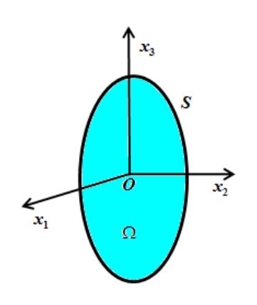
We introduce orthogonal axes of coordinates \(Ox_{1}x_{2}x_{3}\), \(Ox_{3}\) directed vertically upwards.
The heavy viscoelastic fluid occupies a bounded domain \(\Omega\) with regular boundary \(S\) and \(g\) is the constant acceleration of the gravity. The fluid is nonuniformly heated from below.
Figure 1. Model of the system.
The equations of the problem are: taking into account the Boussinesq approximation, the hydrodynamic equations take the form,
\begin{equation}
\label{eq7}
\rho \dot{u}_{i}=-\frac{\partial P}{\partial x_{i}}+\frac{\partial \sigma’_{ij}}{\partial x_{j}}+\rho g \delta T \delta_{i3} \qquad (i,j=1,2,3)
\end{equation}
where \(\vec{u}(t,x)\) is the velocity of the fluid particle from its position at the state of mechanical equilibrium, \(P(t,x)\) is the deviation of pressure from the hydrostatic pressure corresponding to the constant temperature \(T_{\text{m}}\), \(X>0\)
is the coefficient of temperature conductivity.
If we take
\[
\tau_{ij}=\frac{\partial u_{i}}{\partial x_{j}}+
\frac{\partial u_{j}}{\partial x_{i}} \qquad (i,j=1,2,3)
\]
the components of the tensor \(\tau\), we have the components of the tensor \(\sigma’\)
\[
\sigma’_{ij}=\mu \hat{I}_{0}\tau_{ij}
\]
and then
\[
\frac{\partial \sigma’_{ij}}{\partial x_{j}}=
\mu \hat{I}_{0} \frac{\partial \tau_{ij}}{\partial x_{j}}
=\mu \hat{I}_{0} \left( \frac{\partial^{2} u_{i}}{\partial x_{j} \partial x_{j}}+\frac{\partial}{\partial x_{i}}
\left(
\frac{\partial u_{j}}{\partial x_{j}}
\right)
\right)=\mu \hat{I}_{0} \Delta u_{i}
\]
since \(\frac{\partial u_{j}}{\partial x_{j}}=\text{div} \vec{u}=0\). Therefore, the vectorial equation of the motion of the fluid can be written
\begin{equation}
\label{eq10}
\rho \dot{\vec{u}}=-\overrightarrow{\text{grad}}P+\mu \hat{I}_{0} \Delta \vec{u}+\rho g \delta T \vec{x}_{3}
\end{equation}
(10)
We add the stickiness condition
\begin{equation}
\label{eq11}
\vec{u}=0 \qquad \text{on}\;\; S
\end{equation}
(11)
Now we will give boundary condition for the temperature.
5. Conditions of mechanical equilibrium
There exist conditions of heating such that the system is in the state of mechanical equilibrium: \(\vec{u}=0\).
(But, then, there is no thermodynamic equilibrium, the temperature varying with the coordinates).
Setting
\[
\vec{u}(t,x)=0;\qquad P=p_{0}(x);\qquad T=T_{0}(x),
\]
we obtain
\[
\overrightarrow{\text{grad}}p_{0}=\rho g \delta T_{0} \vec{x}_{3};\qquad \Delta T_{0}=0
\]
\(p_{0}\) and \(T_{0}\) are functions of \(x_{3}\) only and we have
\[
\frac{\text{d}^2 T_{0}}{\text{d}x^{2}_{3}}=0
\]
i.e
\[
T_{0}=-\tilde{\alpha}x_{3}+\tilde{\alpha}_{0} \qquad (\tilde{\alpha}\;\;, \tilde{\alpha}_{0}\; \text{constants}).
\]
In the following, we consider the case \(\tilde{\alpha}>0\), corresponding to the heating from below.
The pressure in the state of mechanical equilibrium is given by
\[
\frac{\text{d}p_{0}}{\text{d}x_{3}}=\rho g \delta(-\tilde{\alpha}x_{3}+\tilde{\alpha}_{0})
\]
i.e
\[
p_{0}(x_{3})=\rho g \delta
\left(-\tilde{\alpha}\frac{x^{2}_{3}}{2}+\tilde{\alpha}_{0}x_{3} \right)+\text{constant}
\]
Concerning the boundary condition for the temperature, we suppose [2] that the temperature remain equal to \(T_{0}\) on the wall \(S\), so that, if we set
\[
\theta(t,x)=T(t,x)-T_{0}(x_{3})
\]
we have
\begin{equation}
\label{eq12}
\theta=0 \qquad \text{on}\;\; S
\end{equation}
(12)
6. Final formulation of the problem
Supposing the existence of the previous state of mechanical equilibrium, we seek the solutions of the equations in the form
\[
\vec{u}=\vec{u}(t,x);\qquad P=p_{0}(x_{3})+p(t,x);\qquad T=T_{0}(x_{3})+ \theta(t,x)
\]
where \(\vec{u} \;, p\;, \theta\) are of the first order infinitesimal.
We get
where \(\nu=\frac{\mu}{\rho}\) being the kinematic coefficient of viscosity. The equations (8), (11), (12) remains unchanged.
7. Transition to a system of operatorial equations
(1) We are going to seek \(\vec{u}(t,x),\; p(t,x)\), \(\theta (t,x)\) functions of \(t\) with values in \(J^{1}_{0}(\Omega)\), \(H^{1}(\Omega)\), \(H^{1}_{0}(\Omega)\) respectively, where
\[
J^{1}_{0}(\Omega)=\left\{
\vec{u} \in \left[ H^1(\Omega)\right]^3;\;\; \text{div}\vec{u}=0 \;\; ; \;\; \vec{u}_{|S}=0
\right\}
\]
We introduce the space
\[
J_{0}(\Omega)=\left\{
\vec{u} \in \mathcal{L}^2(\Omega) \overset{\text{def}}{=} \left[ L^2(\Omega)\right]^3;\;\; \text{div}\vec{u}=0\;\; ;\; u_{n|S}=0
\right\},
\]
where \(u_{n|S}\) is the external normal component of \(\vec{u}\) on \(S\).\\
It is well-known [4] that the embedding from \(J^{1}_{0}(\Omega)\) into \(J_{0}(\Omega)\) is continuous, dense and compact and that we have the orthogonal decomposition
The first integral of the right-hand side is equal to zero, because \( \overrightarrow{\text{grad}}p \in \mathcal{G} \left(\Omega \right)\) and \(\vec{\tilde{u}} \in J^{1}_{0}(\Omega) \subset J_{0}(\Omega) \).
The vectorial Laplacian formula [4] can be written by setting \( \epsilon_{ij}=\frac{1}{2}\tau_{ij}\) as
\[
\int_\Omega \, \Delta {\vec{u}} \cdot \bar{\vec{\tilde{u}}}
\, \mathrm d\Omega=
-2\int_\Omega \,\epsilon_{ij}(\vec{u})\epsilon_{ij}(\bar{\vec{\tilde{u}}})+
2\int_S \,\epsilon_{ij}(\vec{u})n_{j}\bar{\tilde{u}}_{i}
\, \mathrm dS
\]
and the last integral is equal to zero by virtue of (11).
It is well-known that
\[
\left( 2\int_\Omega \,\epsilon_{ij}(\vec{u})\epsilon_{ij}(\bar{\vec{u}})
\, \mathrm d\Omega \right)^{1/2}
\]
defines a norm on \(J^{1}_{0}(\Omega)\), that is equivalent to the classical norm of \( \left[ H^{1}(\Omega) \right]^{3}\).
We denote by \(A_{0}\) the unbounded operator of \(J_{0}(\Omega)\) associated to the pair \((J^{1}_{0}(\Omega),J_{0}(\Omega)) \) and to this norm.
Finally, denoting by \(P_{0}\), the orthogonal projector from \(\mathcal{L}^2(\Omega)\) into \(J_{0}(\Omega)\), we can write
\[
\left( \delta g \theta \vec{x}_{3},\vec{\tilde{u}} \right)_{\mathcal{L}^2(\Omega)}=
\left(P_{0} ( \delta g \theta \vec{x}_{3}) ,\vec{\tilde{u}}\right)_{J_{0}(\Omega)}
\]
So, the variational equation (16) is equivalent to the operatorial equation [5]
\begin{equation}
\label{eq17}
\dot{\vec{u}}+\nu \hat{I}_{0} A_{0}\vec{u}-\delta g
P_{0} (\theta \vec{x}_{3})=0
\end{equation}
(17)
(2) In the same manner, for every \(\tilde{\theta} \in H^{1}_{0}(\Omega)\), we have
Since \(\tilde{\theta}|_{S}=0\), the Green formula gives
\[
\int_\Omega \,\Delta \theta \cdot \bar{\tilde{\theta}} \, \mathrm d\Omega =-\int_\Omega \,\overrightarrow{\text{grad}} \theta \cdot \overrightarrow{\text{grad}}\bar{\tilde{\theta}} \, \mathrm d\Omega
\]
It is well-known that \((\int_\Omega \,|\overrightarrow{\text{grad}} \theta |^{2}\, \mathrm d\Omega)^{1/2} \) defines norm a on \( H^{1}_{0}(\Omega)\), that is equivalent to the classical norm of \(H^{1}(\Omega)\). We denote by \(A_{1}\) the unbounded operator of \(L^{2}(\Omega)\) associated to the pair \((H^{1}_{0}(\Omega), L^{2}(\Omega))\) and to this norm.
So the variational equation (18) is equivalent to the operatorial equation [5]
(3) By setting [2]
\[
\theta (t,x)=\left( \frac{\tilde{\alpha}}{\delta g}\right)^{1/2}
w(t,x) ; \qquad \epsilon=(\tilde{\alpha} \delta g)^{1/2}
\]
The equations (17) and (19) take the form
\begin{equation}
\label{eq20}
\dot{\vec{u}}+\nu \hat{I}_{0} A_{0}\vec{u}-\epsilon
P_{0} (w \vec{x}_{3})=0
\end{equation}
(4) Now, we aim to replace the equation (20) by two equations whose coefficients do not depend on \(t \) [2].
As
\[
\hat{I}_{0} A_{0}\vec{u}=A_{0}\vec{u}(t,x)+\alpha \int_{0}^{t}
e^{-\gamma(t-s)}A_{0}\vec{u}(s,x)
\, \mathrm ds
\]
By setting
\[
\vec{u}_{0}(t,x)=\vec{u}(t,x); \qquad \vec{u}_{1}(t,x)=
(\nu \alpha)^{1/2} \int_{0}^{t}
e^{-\gamma(t-s)}A^{1/2}_{0}\vec{u}(s,x)
\, \mathrm ds
\]
We have
\[
(\nu \alpha)^{1/2} A^{1/2}_{0}\vec{u}(t,x)=
\nu \alpha \int_{0}^{t}
e^{-\gamma(t-s)}A_{0}\vec{u}(s,x)
\, \mathrm ds
\]
and the equation (20) becomes
\begin{equation}
\label{eq22}
\dot{\vec{u}}_{0}+ \nu A_{0}\vec{u}_{0}+(\nu \alpha)^{1/2}A_{0}^{1/2}\vec{u}_{1}-\epsilon P_{0} (w \vec{x}_{3})=0
\end{equation}
(1) We seek the solutions of the equations (22), (23), (21) in the form
\[
\vec{u}_{0}=e^{-\lambda t}\vec{u}_{0}(x) \, ;\qquad
\vec{u}_{1}=e^{-\lambda t}\vec{u}_{1}(x)\, ;\qquad
w=e^{-\lambda t}w(x)
\, ;\qquad \lambda \in \mathbb{C}
\]
We obtain
\begin{equation}
\label{eq26}
-\epsilon \vec{u}_{0}\cdot\vec{x}_{3} +XA_{1}w=\lambda w
\end{equation}
(26)
It is easy to verify that \(\lambda =\gamma\) is not an eigenvalue.
Indeed, if \(\lambda =\gamma\), (25) gives \(\vec{u}_{0}=0\), then (26) gives
$$A_{1}w=\frac{\gamma }{X}w $$and consequently \(w=0\), if dismiss the exceptional case where
\(\frac{\gamma }{X}\) is an eigenvalue of \(A_{1}\); finally, (24) gives \(\vec{u}_{1}=0\).
Therefore, we have
\[
\vec{u}_{1}=-\frac{(\nu \alpha)^{1/2} A_{0}^{1/2}\vec{u}_{0}}{\lambda – \gamma}
\]
so that, taking (3) into account, the equation (24) takes the form
\[
\nu I_{0}(\lambda)A_{0}\vec{u}_{0}-\epsilon P_{0}(w\vec{x}_{3})=\lambda \vec{u}_{0}
\]
Let us introduce the operators \(C\) from \(L^2(\Omega)\) into \(J_{0}(\Omega)\) and \(C^{\ast}\) from \(J_{0}(\Omega)\) into \(L^2(\Omega)\) defined by
\[
Cw=P_{0}(w\vec{x}_{3}) \qquad;\qquad C^{\ast}\vec{u}=\vec{u}\cdot \vec{x}_{3}
\]
It is easy to verify that these operators are bounded, with a norm smaller that one, and mutually adjoints.
Since \(\vec{u}_{0}=\vec{u}\), we obtain the equations of the normal oscillations in the form
\begin{equation}
\label{eq27}
\nu I_{0}(\lambda)A_{0}\vec{u}-\epsilon C w=\lambda \vec{u}
\end{equation}
(27)
\begin{equation}
\label{eq28}
-\epsilon C^{\ast}\vec{u}+XA_{1}w =\lambda w
\end{equation}
(28)
(2) We can deduce from Equations (27), (28)
with bounded coefficients by setting
\[
A_{0}^{1/2}\vec{u}=\vec{U}\in J_{0}(\Omega);\qquad
A_{1}^{1/2}w=V\in L^{2}(\Omega)
\]
and by applying the operators \(A_{0}^{-1/2} \) and \(A_{1}^{-1/2} \) to the equations (27), (28) respectively.
Setting
\[
D=A_{0}^{-1/2} C A_{1}^{-1/2};\qquad D^{\ast}=A_{1}^{-1/2} C^{\ast} A_{0}^{-1/2}
\]
we obtain
\begin{equation}
\label{eq30}
-\epsilon D^{\ast}\vec{U}+XV =\lambda A_{1}^{-1/2} V
\end{equation}
(30)
It is easy to see that \(D\) and \(D^{\ast}\) are mutually adjoint and compact.
9. Existence and symmetry of the spectrum
We write the equations (29) and (30) in the form
\[
\mathbf{J} \begin{pmatrix}
\vec{U} \\
V
\end{pmatrix}
+
\begin{pmatrix}
0 &-\epsilon D \\
-\epsilon D^{\ast} & 0
\end{pmatrix}
\begin{pmatrix}
\vec{U} \\
V
\end{pmatrix}
-\lambda
\begin{pmatrix}
A_{0}^{-1} &0 \\
0 & A_{1}^{-1}
\end{pmatrix}
\begin{pmatrix}
\vec{U} \\
V
\end{pmatrix}
=0
\]
where
\[
\mathbf{J}=
\begin{pmatrix}
\nu I_{0}(\lambda)I_{J_{0}(\Omega) } &0 \\
0 & XI_{L^{2}(\Omega)}
\end{pmatrix}
\]
has an inverse and
\[
\begin{pmatrix}
\vec{U} \\
V
\end{pmatrix} \in \chi \overset{\text{def}}{=}
J_{0}(\Omega)\oplus L^{2}(\Omega)
\]
Applying \(\mathbf{J}^{-1}\), we obtain
\begin{equation*}
\left\{
\begin{array}{l}
I_{\chi} \begin{pmatrix}
\vec{U} \\
V
\end{pmatrix}
+
\begin{pmatrix}
0 &\nu^{-1} I_{0}(\lambda)^{-1}\epsilon D \\
-X^{-1}\epsilon D^{\ast} & 0
\end{pmatrix}
\begin{pmatrix}
\vec{U} \\
V
\end{pmatrix}\\[.2cm]
\\[.2cm]
-\lambda
\begin{pmatrix}
\nu^{-1} I_{0}(\lambda)^{-1}A_{0}^{-1} &0 \\
0 & X^{-1} A_{1}^{-1}
\end{pmatrix}
\begin{pmatrix}
\vec{U} \\
V
\end{pmatrix}
=0
\\[.2cm]
\end{array}
\right.
\end{equation*}
that has the form
\[
\left( I_{\chi} +\Phi (\lambda) \right)\begin{pmatrix}
\vec{U} \\
V
\end{pmatrix}=0
\]
where \(\Phi(\lambda)\) is a operatorial function with compact values.
Consequently, we obtain a Fredholm pencil in \(\mathbb{C}-\left\lbrace\beta \right\rbrace\), since \(\beta\) is a pole of \(I_{0}(\lambda)^{-1}\). This pencil is regular, then since \(\lambda=\gamma\) is not an eigenvalue, \(I+\Phi(\lambda)\) has a bounded inverse [4].
Then, the spectrum of the problem exists and consists of isolated points and its accumulation points may be located in
\(\lambda=\beta\) and \(\lambda=\infty\). All points of the spectrum are eigenvalues and the corresponding eigenelements have finite multiplicities.
On the other hand, it is obvious that the initial pencil is self adjoint, so that the spectrum is symmetrical with respect to the real axis.
10. Location of the spectrum in the complex right half-plane
i.e. if \(\nu \) and \(X\) are sufficiently large, we have
\[
\Re \lambda >0
\]
so that the system is stable.
11. Existence of a set of positive real eigenvalues having \(\lambda =\beta\) as point of accumulation
The equation (30) can be written as
\[
\left( X I_{L^{2}(\Omega)}-\lambda A_{1}^{-1} \right)V+\epsilon D^{\ast} \vec{U}=0
\]
\(A_{1}^{-1}\) has a denumerable infinity of positive real eigenvalues, the largest being \( \left\| A_{1}^{-1} \right\|\). Consequently, \( XI_{L^{2}(\Omega)}-\lambda A_{1}^{-1}\) has a bounded inverse if \(\lambda\) is not real and if \(\lambda\) is real with \(\left|\lambda\right|< \frac{X}{ \left\| A_{1}^{-1} \right\|}\). Under this condition, we have
\[
V=-\epsilon \left(XI_{L^{2}(\Omega)}-\lambda A_{1}^{-1} \right)^{-1}D^{\ast}\vec{U}
\]
Carrying out in the equation (29), we obtain
\[
\nu I_{0}(\lambda) \vec{U}+\epsilon^{2}D\left(XI_{L^{2}(\Omega)}-\lambda A_{1}^{-1} \right)^{-1}D^{\ast}\vec{U}-\lambda A_{0}^{-1}\vec{U}=0
\]
If \(X\) is sufficiently large, the inequality \(\left|\lambda\right|< \frac{X}{ \left\| A_{1}^{-1} \right\|}\) is satisfied for \(\lambda=\beta\) and for \(\lambda\) sufficiently close to
\(\beta\).
Setting
\[
\lambda=\lambda’+\beta,\qquad \left|\lambda’\right|\text{ sufficiently small}
\]
we obtain the equation
\(\mathcal{L}(\lambda’)\) is an operatorial function holomorphic in the vicinity of \(\lambda’=0\) and self adjoint.
We have
\[
\mathcal{L}(0)=
\epsilon^{2}D\left(XI_{L^{2}(\Omega)}-\beta A_{1}^{-1} \right)^{-1}D^{\ast}-\beta A_{0}^{-1}
\]
that is compact.\\
Calculating the derivative, we obtain
\[
\mathcal{L}'(0)=
\frac{\nu}{\beta-\gamma}I_{J_{0}(\Omega)}
+\epsilon^{2}D \left[ XI_{L^{2}(\Omega)}-\beta A_{1}^{-1} \right]^{-1}A_{1}^{-1}\left[ XI_{L^{2}(\Omega)}-\beta A_{1}^{-1} \right]^{-1} D^{\ast}
– A_{0}^{-1}
\]
that is strongly positive if \(\nu\) is sufficiently large.
So, [4], if \(\nu\) and \(X\) are sufficiently large, for each \(\eta>0\) sufficiently small, there exists in \(]\beta-\eta,\beta+\eta [\) a set of real eigenvalues of the spectrum of the problem having \(\beta\) as point of accumulation.
12. Location of the non real eigenvalues
We consider a non real eigenvalue \(\lambda\) and
\(
\begin{pmatrix}
\vec{U} \\
V
\end{pmatrix}
\)
an associated eigenelement.
The equations (29) and (30) can be written
\[
\left\{
\begin{array}{l}
\nu \frac{I_{0}(\lambda)}{\lambda} \vec{U} – \frac{\epsilon}{\lambda} DV=A_{0}^{-1} \vec{U}
\\[.2cm]
\\[.2cm]
-\frac{\epsilon}{\lambda}D^{\ast}\vec{U}+\frac{X}{\lambda}VI_{L^{2}(\Omega)}=A_{1}^{-1} V
\\[.2cm]
\end{array}
\right.
\]
From these equations, we deduce
\[
\left\{
\begin{array}{l}
\nu \frac{I_{0}(\lambda)}{\lambda} \left\|\vec{U} \right\|_{J_{0}(\Omega)}^2
– \frac{\epsilon}{\lambda} \left(DV, \vec{U} \right)_{J_{0}(\Omega)}=\left(A_{0}^{-1} \vec{U}, \vec{U} \right)_{J_{0}(\Omega)}
\\[.2cm]
\\[.2cm]
-\frac{\epsilon}{\bar{\lambda}}\left(DV, \vec{U} \right)_{J_{0}(\Omega)}+\frac{X}{\bar{\lambda}}\left\| V \right\|_{L^{2}(\Omega)}^2=\left(A_{1}^{-1} V, V \right)_{L^{2}(\Omega)}
\\[.2cm]
\end{array}
\right.
\]
and then
\[
\frac{\nu}{\epsilon} \Im \frac{I_{0}(\lambda)}{\lambda} \left\|\vec{U} \right\|_{J_{0}(\Omega)}^2
-\frac{X}{\epsilon}\Im \frac{1}{\bar{\lambda}} \left\| V \right\|_{L^{2}(\Omega)}^2
=-\frac{2 \Im \lambda}{\left|\lambda\right|^{2}} \Re \left(DV, \vec{U} \right)_{J_{0}(\Omega)}
\]
Calculating \( \Im \frac{I_{0}(\lambda)}{\lambda}\) and dividing by \(\Im \lambda \neq 0\), we obtain
\[
\frac{\nu}{2}\left\|\vec{U} \right\|_{J_{0}(\Omega)}^2 \left[
\frac{\frac{\beta-\gamma}{\gamma}}{\left|\lambda-\gamma\right|^{2}}-\frac{\frac{\beta}{\gamma}}{\left|\lambda\right|^{2}}
\right]
-\frac{X}{\epsilon} \frac{1}{\left|\lambda\right|^{2}}
\left\| V \right\|_{L^{2}(\Omega)}^2
=
-\frac{2}{\left|\lambda\right|^{2}}
\Re \left(DV, \vec{U} \right)_{J_{0}(\Omega)}
\]
or, using (32)
\[
\left\{\frac{\nu}{2}\left[
\frac{\frac{\beta-\gamma}{\gamma}}{\left|\lambda-\gamma\right|^{2}}-\frac{\frac{\beta}{\gamma}}{\left|\lambda\right|^{2}}
\right]+\frac{\left\| A_{0}^{-1} \right\|}{\left|\lambda\right|^{2}}
\right\}\left\|\vec{U} \right\|_{J_{0}(\Omega)}^2
\geq
\frac{1}{\left|\lambda\right|^{2}} \left[
\frac{X}{\epsilon}-\left\| A_{1}^{-1} \right\|
\right]\left\| V \right\|_{L^{2}(\Omega)}^2
\]
The right-hand side of above equation is positive according to (33), so that the eventual nonreal eigenvalues must verify
with
\[
k=\frac{\frac{\nu}{\epsilon} \cdot \frac{\beta}{\gamma}-\left\| A_{0}^{-1} \right\|}{\frac{\nu}{2} \cdot \frac{\beta-\gamma}{\gamma}}
\]
which is greater than \(1\) according to (33).
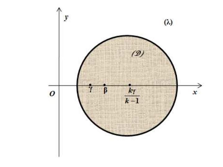
Setting \(\lambda=x+iy\), we see that the domain of the complex plane \((\lambda)\) defined by (35) is the disk \(\mathcal{D}\) defined by
\[
\left(x-\frac{k\gamma}{k-1} \right)^2+y^{2}< \frac{k\gamma^{2}}{(k-1)^2}
\]
\(\lambda=\gamma\) belongs to \(\mathcal{D}\) and it is easy to verify that \(\lambda =\beta\) belongs to \(\mathcal{D}\).
Figure 2. Location of the non real eigenvalues.
13. Reduction to a Krein – Langer pencil
(1) Multiplying the equations 29) and (30) by \(\lambda – \gamma \neq 0\), we obtain
(2) Let us study the properties of the operators of the equation (38).
(a) \(\mathcal{\tilde{C}}\) is obviously self adjoint, positive definite, compact.
(b) \(\mathbf{\tilde{B}}\) is bounded and self adjoint.
We have
\[
\begin{aligned}
&\left(\mathbf{\tilde{B}} z, z \right)_{\chi}
= \nu \left\| \vec{U}\right\|^{2}_{J_{0}(\Omega)}
+X\left\| V\right\|^{2}_{L^{2}(\Omega)}
+\gamma \left[ \left(A_{0}^{-1} \vec{U}, \vec{U} \right)_{J_{0}(\Omega)}
+\left(A_{1}^{-1} V, V \right)_{L^{2}(\Omega)} \right] \\
& \qquad \qquad \qquad -2\epsilon \Re \left(DV, \vec{U} \right)_{J_{0}(\Omega)}
\end{aligned}
\]
Using the inequality (32), we obtain
\[
\begin{aligned}
&\left(\mathbf{\tilde{B}} z, z \right)_{\chi}
\geq \left( \nu -\epsilon \left\| A_{0}^{-1} \right\| \right) \left\| \vec{U}\right\|^{2}_{J_{0}(\Omega)}
+ \left( X -\epsilon \left\| A_{1}^{-1} \right\| \right)\left\| V\right\|^{2}_{L^{2}(\Omega)}
\\
& \qquad \qquad \qquad + \gamma \left[ \left(A_{0}^{-1} \vec{U}, \vec{U} \right)_{J_{0}(\Omega)}
+\left(A_{1}^{-1} V, V \right)_{L^{2}(\Omega)} \right]
\end{aligned}
\]
By virtue of the inequalities (33), \(\mathbf{\tilde{B}}\) is strongly positive.
(c) \( \mathbf{Q}\) is bounded and self adjoint.
On the other hand, we have
\[
\begin{aligned}
&\left(\mathbf{Q} z, z \right)_{\chi}
\geq \nu \left( \beta-\gamma \right)\left\| \vec{U}\right\|^{2}_{J_{0}(\Omega)}
\\
& \qquad \qquad \qquad + \gamma \left[ \left( \nu -\epsilon \left\| A_{0}^{-1} \right\| \right) \left\| \vec{U}\right\|^{2}_{J_{0}(\Omega)}
+ \left( X -\epsilon \left\| A_{1}^{-1} \right\| \right)\left\| V\right\|^{2}_{L^{2}(\Omega)} \right]
\end{aligned}
\]
so that \(\mathbf{Q}\) is strongly positive and then admits an inverse that has the same properties.
(3) Setting
\[
\mathbf{Q}^{1/2}z=W\in \chi
\]
carrying out in (38) and applying \(\mathbf{Q}^{-1/2}\), we obtain
\[
W+\tilde{\lambda}\mathbf{Q}^{-1/2} \mathbf{\tilde{B}} \mathbf{Q}^{-1/2}W+ \tilde{\lambda}^{2}\mathbf{Q}^{-1/2} \mathcal{\tilde{C}} \mathbf{Q}^{-1/2}W=0
\]
It is easy to see that \(\mathbf{B} =\mathbf{Q}^{-1/2} \mathbf{\tilde{B}} \mathbf{Q}^{-1/2}\) and
\(\mathcal{C}=\mathbf{Q}^{-1/2} \mathcal{\tilde{C}} \mathbf{Q}^{-1/2}\) are bounded, self adjoint and positive definite and \(\mathcal{C}\) is compact.
So we obtain a Krein-Langer pencil [2; pp 295-309]
\begin{equation}
\label{eq39}
\hat{L}(\tilde{\lambda}) \overset{\text{def}}{=} I + \tilde{\lambda}\mathbf{B}+\tilde{\lambda}^{2}\mathcal{C}
\end{equation}
(39)
(4) The theory of this pencil is treated in [3]. We restrict ourselves to an additional result.
Since \(\mathbf{B}\) is self adjoint, the set of the nonreal eigenvalues may have only the infinity as point of accumulation.
Consequently, since these eigenvalues are in the disk \(\mathcal{D}\), there are no more than a finite number of such eigenvalues.
14. Existence and unicity of the solution of the associated evolution problem
We write the equations (22), (23), (21)
in the form
\[
\dot{\mathbf{W}}+\mathcal{A} \mathbf{W}=0
\]
with
\[
\mathbf{W}=
\begin{pmatrix}
\vec{u}_{0}\\
\vec{u}_{1} \\
w
\end{pmatrix}
\qquad , \quad
\mathcal{A}=
\begin{pmatrix}
\nu A_{0} & (\nu \alpha)^{1/2}A^{1/2}_{0} & -\epsilon C \\
-(\nu \alpha)^{1/2}A^{1/2}_{0} & \gamma I_{J_{0}(\Omega)} & 0 \\
-\epsilon C^{\ast} & 0 & XA_{1}
\end{pmatrix}
\]
We are going to consider \(\mathcal{A}\) as unbounded operator of
\[
H=J_{0}(\Omega)\oplus J_{0}(\Omega) \oplus L^{2}(\Omega)
\]
with domain
\[
D(\mathcal{A})=D(A_{0})\oplus D(A^{1/2}_{0}) \oplus D(A_{1})
\]
We are going to prove that \(-\mathcal{A}\) is maximal dissipative.
(1) \(\mathcal{A}\) is obviously closed.
By direct calculations, we have
\[
\begin{aligned}
&
\left(\mathcal{A} \mathbf{W}, \mathbf{W} \right)_{H}=
\nu \left(A_{0} \vec{u}_{0}, \vec{u}_{0}\right)_{J_{0}(\Omega)}
+\gamma \left\| \vec{u}_{1}\right\|^{2}_{J_{0}(\Omega)}
+X \left(A_{1} w, w \right)_{L^{2}(\Omega)}
-2\epsilon \Re \left(Cw, \vec{u}_{0}\right)_{J_{0}(\Omega)}\\
& \qquad \qquad \qquad +2i\Im \left(A^{1/2}_{0} \vec{u}_{1}, \vec{u}_{0}\right)_{J_{0}(\Omega)}
\end{aligned}
\]
so that
\[
\Re \left(\mathcal{A} \mathbf{W}, \mathbf{W} \right)_{H} \geq 0 \qquad \forall \mathbf{W}\in D(\mathcal{A})
\]
under the condition (33).
(2) We have
\[
\mathcal{A}^{\ast}=
\begin{pmatrix}
\nu A_{0} & -(\nu \alpha)^{1/2}A^{1/2}_{0} & -\epsilon C \\
(\nu \alpha)^{1/2}A^{1/2}_{0} & \gamma I_{J_{0}(\Omega)} & 0 \\
-\epsilon C^{\ast} & 0 & XA_{1}
\end{pmatrix}
\]
so that, in the same manner, we have
\[
\Re \left(\mathcal{A}^{\ast} \mathbf{W}, \mathbf{W} \right)_{H} \geq 0 \qquad \forall \mathbf{W}\in D(\mathcal{A}^{\ast})=D(\mathcal{A})
\]
Consequently, [3;p 54,55], if the initial value \(\mathbf{W}(0)\in D(\mathcal{A})\), i.e
\[
\vec{u}_{0}(0)\in D(A_{0}) \qquad,\qquad
\vec{u}_{1}(0)\in D(A^{1/2}_{0}) \qquad,\qquad
w(0)\in D(A_{1})
\]
the evolution problem has a solution and only one belonging to \(D(\mathcal{A})\) for \(t\geq 0\).
Acknowledgment
The authors are grateful to the referee and the
editorial board for some useful comments that
improved the presentation of the paper.
Author Contributions
All authors contributed equally to the writing of this paper. All authors read and approved the
final manuscript.
Competing Interests
The author(s) do not have any competing interests in the manuscript.
References
Chandrasekhar, S. (2013). Hydrodynamic and hydromagnetic stability. Dover pubications, Inc. New York.
[Google Scholor]
Kopachevsky, N. D., & Krein, S. (2003). Operator Approach to Linear Problems of Hydrodynamics: Volume 2: Nonself-adjoint Problems for Viscous Fluids (Vol. 146). Birkhäuser.[Google Scholor]
Israil’Cudikovic Gochberg, Krejn, M. G. E., & Roos, G. (1971). Introduction à la théorie des opérateurs linéaires non auto-adjoints dans un espace hilbertien. Dunod.[Google Scholor]
Kopachevsky, N. D., & Krein, S. (2001). Operator Approach to Linear Problems of Hydrodynamics: Volume 1: Nonself-adjoint Problems for Viscous Fluids (Vol. 146). Birkhäuser.[Google Scholor]
Lions, J. L. (2013). Equations differentielles operationnelles: et problémes aux limites (Vol. 111). Springer-Verlag.[Google Scholor]