In this paper, we study a new distribution called the exponentiated transmuted Lindley distribution. The proposed distribution has three special cases namely Lindley, exponentiated Lindley and transmuted Lindley distributions. Along with the basic properties of the distribution, the maximum likelihood technique of estimating the parameters of the distribution are discussed. Two applications of the distribution are also part of this article.
Probability distributions are of paramount importance in many practical applications of statistics. In deed, several statistical methods are applicable when the data under consideration follow certain distributions. In a study, one may find a particular probability distribution useful in modelling a data set while in another study a different distribution may be required. The Lindley distribution is among the widely used distributions. It is mainly used to model lifetime data.
Ghitany et al.[1] demonstrated the superiority of the Lindley distribution over the exponential distribution in modelling waiting time data of 100 customers in a bank.
Another important application of the this distribution is the analysis of time series data. Popovi\(\acute{c}\) et al. [2] introduced and showed the application of the autoregressive process of order one with Lindley marginal distribution.
Generalizations of several distributions are available in the statistical science literature. According to Fatima et al. [3], distributions are generalized so as to provide better fits to data and obtain more flexible models. Two common methods of generalizing distributions are the exponentiation method and quadratic rank transmutation map method. The generalized Lindley distribution introduced by Nadarajah et al. [4], was fitted to relief times of twenty patients and compared to Weibull, gamma, and lognormal distribution. The authors concluded that the generalized distribution provided better fits than the other three distributions. Merovci [5] introduced and determined properties of the transmuted Lindley distribution. His data analysis based on this distribution and remission times of 128 cancer patients showcased the superiority of the distribution over the exponential and Lindley distributions, which were all fitted to the data. Other Lindley-type distributions that have been fitted to the data include a new generalization of the transmuted Lindley distribution of Mansour et al.[6] and transmuted two-parameter Lindley distribution of Kemaloglu et al. [7]. According
to Kemaloglu et al., the latter provided better fits to the data than any of Lindley and transmuted power Lindley distributions. Granzotto et al. [8] developed the transmuted power lindley distribution and showed that it can provide better fits to monthly rainfall data than the Lindley, power Lindley, weighted Lindley and transmuted Lindley distributions.
In some situations, an exponentiated transmuted distribution, which is a generalization of a baseline distribution using both exponentiation and transmutation techniques outperforms its special cases [9, 10, 11]. On this note, we propose and study the properties of the exponentiated transmuted Lindley distribution (\(ETLD\)). Suppose there are \(\alpha\) transmuted Lindley variables representing failure times of a component of a system, assumed to be independent. Another motivation for introducing the distribution is that it can be used to determine the probability that the system will fail before a given time. Again, the hazard rate function of the distribution is quite flexible, assuming various shapes, especially non monote shapes. Thus, the distribution will be of use in many practical applications of statistics.
2. The proposed distribution
From the work of Merovci [5], it is obvious that if a random variable \((X)\) has a transmuted Lindley distribution with parameters \(\theta\) and \(\lambda\), then its probability density function (pdf) is
Given that \(x>0, \alpha >0, \theta >0\) and \( \begin{vmatrix}
\lambda
\end{vmatrix} \le 1\), the cdf of the exponentiated transmuted Lindley (ETL) distributed random variable \((X)\)
becomes
The \(ETLD\) is actually a generalization of each of the Lindley, transmuted Lindley and exponentiated (generalized) Lindley distributions. When \(\lambda=0\) and \(\alpha=1\), the proposed
distribution is basically a Lindley distribution. If \(\alpha=1\), the distribution is the same as the transmuted Lindley distribution. The exponentiated Lindley distribution is a special
of the ETL distribution for which \(\lambda=0\).
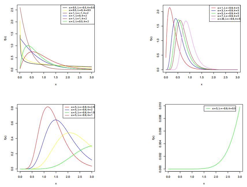
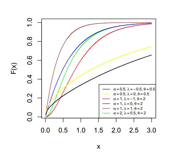
Figures \ref{fig1} and \ref{fig2} show that the pdf and cdf of an exponentiated transmuted Lindley distributed variable may have various shapes, depending
on the values of \(\theta\), \(\lambda\) and \(\alpha\).
Figure 1. pdf of \(ETLD\) for selected values of \(\alpha\), \(\lambda\) and \(\theta\)Figure 2. cdf of \(ETLD\) for selected values of \(\alpha\), \(\lambda\) and \(\theta\)
3. Quantile function
The quantile function \(x_q\) satisfies the equation
To evaluate the raw moment , we may need the series representations
\begin{align}
\left(1-\frac{\theta+1+\theta x}{\theta+1}e^{-\theta x}\right)^{\alpha-1}=\sum_{i=0}^\infty \left(\begin{array}{c} \alpha-1\\ i \end{array}\right)\frac{(-1)^i}{(\theta +1)^{i}}(1+\theta(1+x))^ie^{-\theta ix},
\end{align}
\begin{align}
\left(1+\lambda \frac{\theta+1+\theta x}{\theta+1}e^{-\theta x}\right)^{\alpha-1}=\sum_{j=0}^\infty \left(\begin{array}{c} \alpha-1\\ j \end{array}\right)\frac{\lambda^j}{(\theta +1)^{j}}(1+\theta(1+ x))^{j}e^{-\theta jx},
\end{align}
\begin{align}
\left(1+\theta(1+ x)\right)^{i+j}=\sum_{k=0}^{i+j} \left(\begin{array}{c} i+j\\ k \end{array}\right)\theta ^k(1+ x)^{k}
\end{align}
and
\begin{align}
\left(1+x\right)^{k+1}=\sum_{s=0}^{k+1} \left(\begin{array}{c} k+1\\ s \end{array}\right)x^s.
\end{align}
Thus,
\begin{align}
E(X^r)&= \frac{\alpha \theta ^2}{\theta+1}\sum_{i=0}^\infty\sum_{j=0}^\infty\sum_{k=0}^{i+j}\sum_{s=0}^{k+1} \left(\begin{array}{c} \alpha-1\\ i \end{array}\right)
\left(\begin{array}{c} \alpha-1\\ j \end{array}\right)
\left(\begin{array}{c} i+j\\ k \end{array}\right)\left(\begin{array}{c} k+1\\ s \end{array}\right)\\ &\times\frac{(-1)^i \lambda^j\theta^k}{(\theta+1)^{i+j}}
\int_0^\infty x^{r+s}e^{-\theta(i+j+1) x}\left(1-\lambda+2\lambda\frac{\theta+1+\theta x}{\theta+1}e^{-\theta x}\right)
dx.
\end{align}
The integral
\begin{align*}
&\int_0^\infty x^{r+s}e^{-\theta(i+j+1) x}\left(1-\lambda+2\lambda\frac{\theta+1+\theta x}{\theta+1}e^{-\theta x}\right)
dx\\
&=(1-\lambda)\int_0^\infty x^{r+s}e^{-\theta(i+j+1) x}
dx+2\lambda\int_0^\infty x^{r+s}e^{-\theta(i+j+2) x}
dx+\frac{2\lambda \theta}{\theta+1}\int_0^\infty x^{r+s+1}e^{-\theta(i+j+2) x}dx\\&=\frac{(r+s)!}{\theta^{r+s+1}}\left(\frac{1-\lambda}{(i+j+1)^{r+s+1}}+\frac{2\lambda}{(i+j+2)^{r+s+1}}+\frac{2\lambda (r+s+1)}{(\theta+1) (i+j+2)^{r+s+2}}\right).
\end{align*}
Using the results obtained above, the moment becomes
\begin{align}
E(X^r)&= \frac{\alpha \theta ^2}{1+\theta}\sum_{i=0}^\infty\sum_{j=0}^\infty\sum_{k=0}^{i+j}\sum_{s=0}^{k+1} \left(\begin{array}{c} \alpha-1\\ i \end{array}\right)
\left(\begin{array}{c} \alpha-1\\ j \end{array}\right)
\left(\begin{array}{c} i+j\\ k \end{array}\right)\left(\begin{array}{c} k+1\\ s \end{array}\right)\\ &\times\frac{(-1)^i \lambda^j\theta^k (r+s)!}{(\theta+1)^{i+j}\theta^{r+s+1}}
\left(\frac{1-\lambda}{(i+j+1)^{r+s+1}}+\frac{2\lambda}{(i+j+2)^{r+s+1}}+\frac{2\lambda (r+s+1)}{(\theta+1) (i+j+2)^{r+s+2}}\right).
\end{align}
The moment generating function of the \(ETL\) variable is
\begin{align}
M_X(t)&=E(e^{tX})
\\&=\sum_{\omega=0}^\infty \frac{t^\omega E(X^\omega)}{\omega!}\\
&=\frac{\alpha \theta ^2}{1+\theta}\sum_{\omega=0}^\infty\sum_{i=0}^\infty\sum_{j=0}^\infty\sum_{k=0}^{i+j}\sum_{s=0}^{k+1} \left(\begin{array}{c} \alpha-1\\ i \end{array}\right)
\left(\begin{array}{c} \alpha-1\\ j \end{array}\right)
\left(\begin{array}{c} i+j\\ k \end{array}\right)\left(\begin{array}{c} k+1\\ s \end{array}\right)\\ &\times\frac{(-1)^i \lambda^j\theta^k (\omega+s)!t^\omega}{(\theta+1)^{i+j}\theta^{\omega+s+1}\omega!}
\left(\frac{1-\lambda}{(i+j+1)^{\omega+s+1}}+\frac{2\lambda}{(i+j+2)^{\omega+s+1}}+\frac{2\lambda (\omega+s+1)}{(\theta+1) (i+j+2)^{\omega+s+2}}\right).\end{align}
With the formula for finding \(E(X^r)\), the mean and variance of the \(ETL\) distribution can be determined. The classical coefficients of skewness and kurtosis obtained using the rth raw moment
formula have some weaknesses and are now replaced by the Bowley skewness (\(S\)) [12] and Moors kurtosis (\(K\)) [13] respectively. Consequently,
\begin{align*}
S=\frac{Q(\frac{3}{4})-2Q(\frac{2}{4})+Q(\frac{1}{4})}{Q(\frac{3}{4})-Q(\frac{1}{4})}
\end{align*}
and
\begin{align*}
K=\frac{Q(\frac{7}{8})-Q(\frac{5}{8})+Q(\frac{3}{8})-Q(\frac{1}{8})}{Q(\frac{6}{8})-Q(\frac{2}{8})},
\end{align*} where \(Q(.)\) represents the quantile function.
In Table 1, the mean, median, variance, Bowley skewness and Moors kurtosis are presented for various parameter values of the \(ETLD\) .
We have computed these summary measures in order to examine the relationships between them and the parameters of the \(ETLD\).
Table 1. Some Summary Measures based on \(ETLD\).
\(\alpha\)
\(\lambda\)
\(\theta\)
Mean
Median
Variance
S
K
0.1
0.2
0.5
0.5017
0.0049
1.9904
0.9637
4.2368
0.5
0.2
0.5
1.9281
1.1229
8.9714
0.3213
0.8403
0.9
0.2
0.5
2.8566
2.1517
14.8079
0.2156
0.5776
1.3
0.2
0.5
3.5361
2.8890
19.8520
0.1817
0.4875
1.7
0.2
0.5
4.0693
2.4577
24.3127
0.1648
0.4422
2.1
0.2
0.5
4.5068
3.9192
28.3241
0.1544
0.4147
2.5
0.2
0.5
4.8775
4.3073
31.9777
0.1473
0.3960
2.9
0.2
0.5
5.1986
4.6417
35.3389
0.1422
0.3825
0.5
-0.9
2.5
0.1376
0.3455
0.1102
0.2429
0.6417
0.5
-0.5
2.5
0.1069
0.2474
0.0859
0.3036
0.7859
0.5
-0.1
2.5
0.0850
0.1721
0.0649
0.3835
0.9720
0.5
0.1
2.5
0.0757
0.1451
0.0552
0.4070
1.0475
0.5
0.5
2.5
0.0591
0.1076
0.0371
0.4198
1.1111
0.5
0.9
2.5
0.0446
0.0841
0.0202
0.4083
1.0570
2
-0.1
0.1
27.4823
24.7747
978.2794
0.1305
0.3527
2
-0.1
0.5
4.9569
4.4027
33.2689
0.1351
0.3654
2
-0.1
0.9
2.5640
2.2480
9.1625
0.1418
0.3834
2
-0.1
1.3
1.6847
1.4618
4.0346
0.1482
0.4002
2
-0.1
1.7
1.2380
1.0656
2.2094
0.1535
0.4141
2
-0.1
2.1
0.9713
0.8307
1.3738
0.1579
0.4254
2
-0.1
2.5
0.7955
0.6770
0.9286
0.1613
0.4343
2
-0.1
2.9
0.6716
0.5694
0.6658
0.1640
0.4415
0.1
-0.9
2.5
0.1376
0.0051
0.1102
0.9178
2.6316
0.5
-0.5
2.5
0.4074
0.2474
0.3844
0.3036
0.7859
0.9
-0.1
2.5
0.5044
0.3590
0.4943
0.2447
0.6436
1.3
0.1
2.5
0.5751
0.4395
0.5788
0.2179
0.5786
1.7
0.5
2.5
0.5389
0.4154
0.4961
0.2201
0.5987
2.1
0.9
2.5
0.4469
0.3651
0.3145
0.1845
0.5055
0.1
0.2
0.5
0.5017
0.0049
0.9904
0.9637
4.2368
0.5
0.2
1
0.8487
0.4440
1.8900
0.3716
0.9554
0.9
0.2
1.5
0.7900
0.5455
1.2543
0.2611
0.6898
1.3
0.2
2
0.7086
0.5384
0.8852
0.2218
0.5900
1.7
0.2
2.5
0.6380
0.5089
0.6620
0.2011
0.5367
2.1
0.2
3
0.5797
0.4765
0.5171
0.1880
0.5029
0.5
-0.9
0.5
3.1806
2.4980
17.7535
0.1827
0.4921
0.5
-0.5
1
1.1941
0.7879
3.0667
0.2598
0.6845
0.5
-0.1
1.5
0.6118
0.3299
0.9479
0.3631
0.9160
0.5
0.1
2
0.3921
0.1925
0.4225
0.3999
1.0253
0.5
0.5
2.5
0.2379
0.1076
0.1723
0.4198
1.1112
0.5
0.9
3
0.1433
0.0670
0.0612
0.4113
1.0684
0.1
-0.9
0.5
0.9383
0.0535
4.2448
0.8979
2.1445
0.5
-0.5
1
1.1941
0.7879
3.0667
0.2598
0.6845
0.9
-0.1
1.5
0.9154
0.6720
1.5723
0.2271
0.5999
1.3
0.1
2
0.7450
0.5752
0.9587
0.2118
0.5629
1.7
0.5
2.5
0.5389
0.4154
0.41961
0.2201
0.5987
2.1
0.9
3
0.3609
0.2933
0.2068
0.1878
0.5147
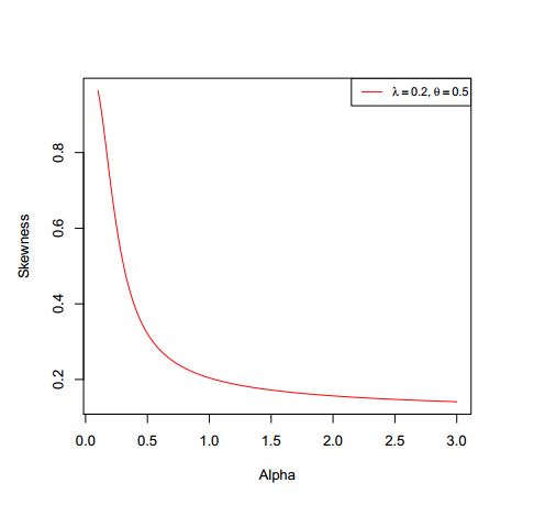
In addition to the numerical results in Table 1, we have provided plots (Figures 3 to 8) to ensure that we make a valid interpretation of the relationship between
each of skewness (S) and kurtosis (K) and any of the parameters when the other two parameters are fixed. From Figures 3 and 4, we conclude that both S and K are nonincreasing
functions of \(\alpha\) if \(\lambda\) and \(\theta\) are fixed.
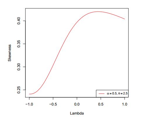
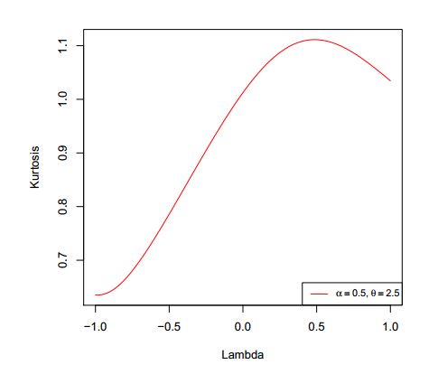
Figures 5 and 6 show that as a function of \(\lambda\) only, each of S and K is unimodal. As shown in Figures 7 and 8, S and K are all
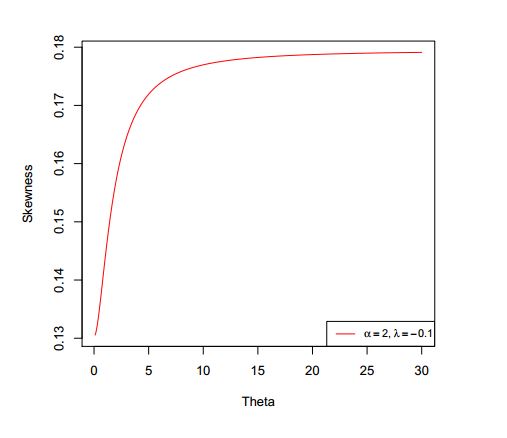
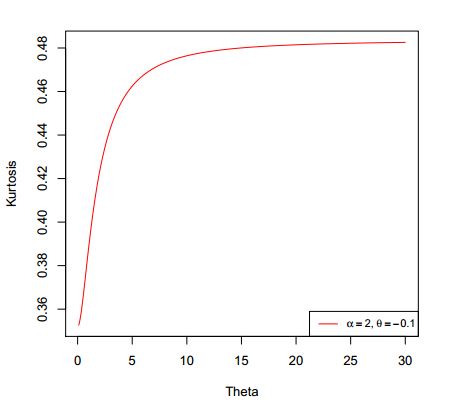
nondecreasing functions of \(\theta\) when \(\alpha\) and \(\lambda\) are fixed. If only \(\alpha\) is held constant, Table 1 indicates that all of the mean, median and
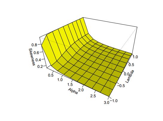
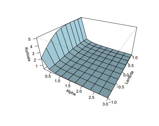
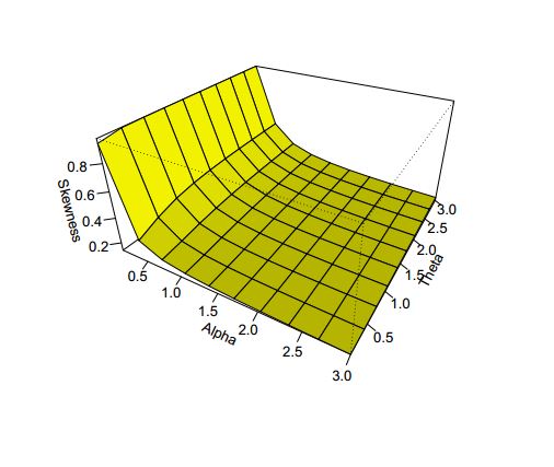
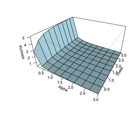
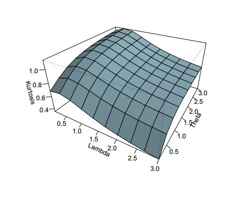
variance increase as \(\lambda\) and \(\theta\) jointly increase. Also, the variance increases provided each of the three parameters increases. Graphs of S and K against
two parameters are displayed in Figures 9 to 14.
Though the results in Table 1 are primarily obtained to investigate some relationships, there also useful in examining whether the distribution is negatively skewed,
symmetric or positively skewed. With the results, we can also determine if the distribution is platykurtic, mesokurtic or leptokurtic.
With regard to the results, distribution is positively skewed and it can be
platykurtic or leptokurtic, depending on the values of the parameters.
Figure 3. Skewness of \(ETLD\) when \(\lambda=0.2\) and \(\theta=0.5\)Figure 4. Kurtosis of \(ETLD\) when \(\lambda=0.2\) and \(\theta=0.5\)Figure 5. Skewness of \(ETLD\) for \(\alpha=0.5\) and \(\theta=2.5\)Figure 6. Kurtosis of ETL distribution \(\alpha=0.5\) and \(\theta=2.5\)Figure 7. Skewness of \(ETLD\) for \(\alpha=2\) and \(\lambda=-0.1\)Figure 8. Kurtosis of \(ETLD\) for \(\alpha=2\) and \(\lambda=-0.1\)Figure 9. Skewness of \(ETLD\) when \(\theta=2.5\)Figure 10. Kurtosis of \(ETLD\) when \(\theta=2.5\)Figure 11. Skewness of \(ETLD\) for \(\lambda=0.2\)Figure 12. Kurtosis of \(ETLD\) for \(\lambda=0.2\)Figure 13. Skewness of \(ETLD\) for \(\alpha=0.5\)Figure 14. Kurtosis of \(ETLD\) for \(\alpha=0.5\)
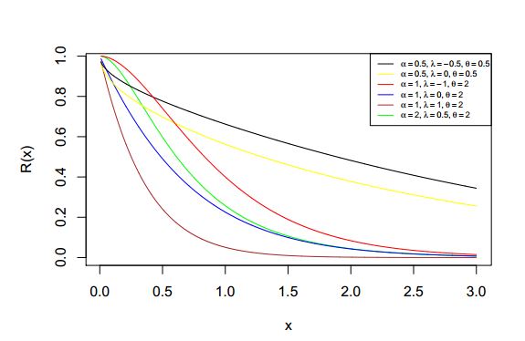
5. Reliability analysis
The reliability function refers to the probability that an item will not fail before a given time \(t\).
In terms of the exponentiated transmuted Lindley distribution with cdf \(F(x)\), this function may be expressed as
Different shapes of the reliability function are graphically shown in Figure 3.
Figure 15. Kurtosis of \(ETLD\) for \(\alpha=0.5\)
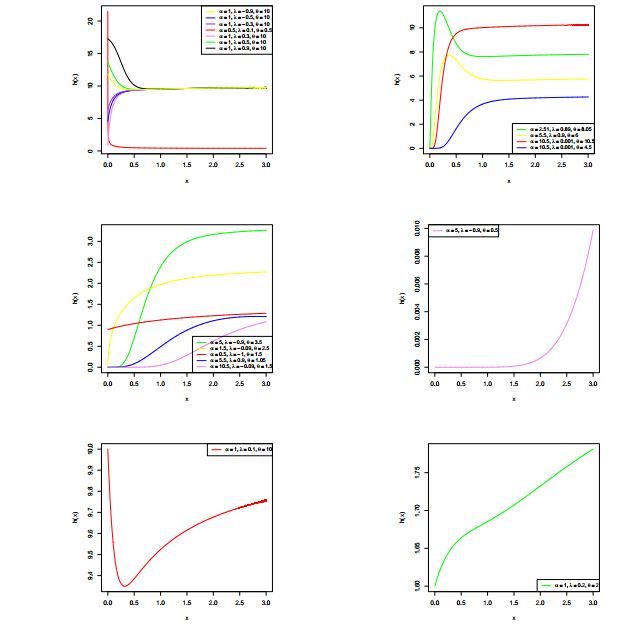
In addition to the reliability function, one’s desire may be to examine the hazard rate function defined by
where \(f(x)\) and \(R(x)\) are defined in (4) and (9) respectively.
Figure 4 is indicative of the effect of parameter value combinations on the shape of the hazard rate function of the \(ETLD\).
Figure 16. Hazard rate function of \(ETLD\) for selected values of \(\alpha\), \(\beta\) and \(\theta\)
6. R\(\acute{\text{e}}\)nyi entropy
The concept of entropy is being used to describe the amount of uncertainty in a random variable.
A popular measure of entropy is the R\(\acute{e}\)nyi entropy, which, for an ETL variable, is defined as
To evaluate (12), we use the series representations:
\begin{align*}
\left(1-\lambda+2\lambda\frac{\theta+1+\theta x}{\theta+1}e^{-\theta x}\right)^\delta=(1-\lambda)^\delta\sum_{a=0}^\infty \begin{pmatrix}
\delta\\
a
\end{pmatrix} \left(\frac{2\lambda}{1-\lambda}\right)^a\left(1+\frac{\theta x}{\theta+1}\right)^a e^{-a\theta x};\\
\left(1-\left(1+\frac{\theta x}{\theta+1}\right)e^{-\theta x}\right)^{(\alpha-1)\delta}=
\sum_{b=0}^\infty \begin{pmatrix}
(\alpha-1)\delta\\
b
\end{pmatrix} (-1)^b \left(1+\frac{\theta x}{\theta+1}\right)^b e^{-b\theta x};\\
\left(1+\lambda\left(1+\frac{\theta x}{\theta+1}\right)e^{-\theta x}\right)^{(\alpha-1)\delta}=
\sum_{c=0}^\infty \begin{pmatrix}
(\alpha-1)\delta\\
c
\end{pmatrix} \lambda^c \left(1+\frac{\theta x}{\theta+1}\right)^c e^{-c\theta x}.
\end{align*}
As a consequence, we obtain
\begin{align}\label{eq13}
I_R(\delta)=\frac{1}{1-\delta}log\int_0^\infty
\begin{pmatrix}
\left(\frac{\alpha \theta ^2}{1+\theta}\right)^\delta (x+1)^\delta (1-\lambda)^\delta \sum_{a=0}^\infty\sum_{b=0}^\infty\sum_{c=0}^\infty\\
\begin{pmatrix}
\delta\\
a
\end{pmatrix}\begin{pmatrix}
(\alpha-1)\delta\\
b
\end{pmatrix} \begin{pmatrix}
(\alpha-1)\delta\\
c
\end{pmatrix}
\left(\frac{2\lambda}{1-\lambda}\right)^a(-1)^b\lambda^c \\\frac{(1+\theta(x+1))^{a+b+c}}{(\theta+1)^{a+b+c}}
e^{-(a+b+c+\delta)\theta x} \end{pmatrix} dx
\end{align}
(13)
With \((1+\theta(x+1))^{a+b+c}=\sum_{d=0}^{a+b+c} \begin{pmatrix}
a+b+c\\
d
\end{pmatrix}\theta^d(x+1)^d\) and \\\((x+1)^{d+\delta}=\sum_{u=0}^\infty\begin{pmatrix}
d+\delta\\
u
\end{pmatrix}x^u\) , (13) can be written as
\begin{align}
I_R(\delta)&=\frac{1}{1-\delta}log
\begin{pmatrix}
\left(\frac{\alpha \theta ^2}{1+\theta}\right)^\delta(1-\lambda)^\delta \sum_{a=0}^\infty\sum_{b=0}^\infty\sum_{c=0}^\infty \sum_{d=0}^{a+b+c}\sum_{u=0}^\infty\\
\begin{pmatrix}
\delta\\
a
\end{pmatrix}\begin{pmatrix}
(\alpha-1)\delta\\
b
\end{pmatrix}\begin{pmatrix}
(\alpha-1)\delta\\
c
\end{pmatrix}\begin{pmatrix}
a+b+c\\
d
\end{pmatrix}\begin{pmatrix}
d+\delta\\
u
\end{pmatrix}\\
\left(\frac{2\lambda}{1-\lambda}\right)^a \frac{(-1)^b\lambda^c\theta^d}{(\theta+1)^{a+b+c}}
\int_0^\infty x^u e^{-(a+b+c+\delta)\theta x} dx
\end{pmatrix} \\
&=\frac{\delta}{1-\delta}log\alpha+\frac{2\delta}{1-\delta}log \theta -\frac{\delta}{1-\delta}log(\theta+1)+\frac{\delta}{1-\delta}log(1-\lambda)\\&
+\frac{1}{1-\delta}log
\begin{pmatrix}
\sum_{a=0}^\infty\sum_{b=0}^\infty\sum_{c=0}^\infty \sum_{d=0}^{a+b+c}\sum_{u=0}^\infty\\
\begin{pmatrix}
\delta\\
a
\end{pmatrix}\begin{pmatrix}
(\alpha-1)\delta\\
b
\end{pmatrix}\begin{pmatrix}
(\alpha-1)\delta\\
c
\end{pmatrix}\begin{pmatrix}
a+b+c\\
d
\end{pmatrix}\begin{pmatrix}
d+\delta\\
u
\end{pmatrix}\\
\left(\frac{2\lambda}{1-\lambda}\right)^a \frac{(-1)^b\lambda^c\theta^d u!}{(\theta+1)^{a+b+c}\theta^{u+1}(a+b+c+\delta)^{u+1}}\end{pmatrix},
\end{align}
(14)
where $$\int_0^\infty x^u e^{-(a+b+c+\delta)\theta x} dx=\frac{u!}{\theta^{u+1}(a+b+c+\delta)^{u+1}}.$$
7. Estimation
The likelihood function of a random sample from the \(ETLD\) with parameters \(\theta, \lambda\) and \(\alpha\) is
\begin{align*}
L&=\prod_{i=1}^n f(x_i;\alpha, \lambda,\theta)\\
&=\left(\frac{\alpha \theta^2}{\theta+1}\right)^n\times\prod_{i=1}^n\begin{pmatrix}
(1+x_i)e^{-\theta x_i}\left(1-\lambda+2\lambda\frac{\theta+1+\theta x_i}{\theta+1}e^{-\theta x_i}\right)\\
\times \left[\left(1-\frac{\theta+1+\theta x_i}{\theta+1}e^{-\theta x_i}\right)\left(1+\lambda\frac{\theta+1+\theta x_i}{\theta+1}e^{-\theta x_i}\right)\right]^{\alpha-1}
\end{pmatrix}
\end{align*}
The log-likelihood function can be written as
\begin{align*}
lnL&=nln\alpha+2nln\theta-nln(\theta+1)+\sum_{i=1}^n ln (x_i+1)-\theta\sum_{i=1}^n x_i\\&+\sum_{i=1}^n ln\left(1-\lambda+2\lambda\frac{\theta+1+\theta x_i}{\theta+1}e^{-\theta x_i}\right) +(\alpha-1) \sum_{i=1}^n ln\left(1-\frac{\theta+1+\theta x_i}{\theta+1}e^{-\theta x_i}\right)\\&
+(\alpha-1)\sum_{i=1}^n ln \left(1+\lambda\frac{\theta+1+\theta x_i}{\theta+1}e^{-\theta x_i}\right).
\end{align*}
Maximum likelihood estimates (MLEs) of the three parameters \(\theta, \lambda\) and \(\alpha\) are determined by solving simultaneously the equations \( \frac{\partial lnL}{\partial \alpha}=0\), \(\frac{\partial lnL}{\partial \lambda}=0\) and \(\frac{\partial lnL}{\partial \theta}=0\). Consequently, the equations \( \frac{\partial lnL}{\partial \alpha}=0\), \(\frac{\partial lnL}{\partial \lambda}=0\) and \(\frac{\partial lnL}{\partial \theta}=0\), are respectively given as
Closed form solution of (15), (16) and (17) cannot be obtained. A numerical approach based on quasi-Newton algorithm may then be used to solve these equations.
Interval estimation of any of the parameters of the ETL distribution is possible when the necessary standard error estimate is known. As \(n\rightarrow\infty\), the MLE
\(\hat{\gamma}=(\hat{\alpha}, \hat{\lambda},\hat{\theta})^{\prime} \) of \(\gamma=(\alpha, \lambda,\theta)^{\prime}\) is asymptotically normally distributed with mean \(\boldsymbol{\gamma}\)
and variance-covariance matrix
$$ V=\begin{pmatrix}{V}_{11}&{V}_{12}&{V}_{13}\\
{V}_{21}&{V}_{22}&{V}_{23}\\
{V}_{31}&{V}_{32}&{V}_{33}
\end{pmatrix}=
\begin{pmatrix}
B_{11}&B_{12}&B_{13}\\
B_{21}&B_{22}&B_{23}\\
B_{31}&B_{32}&B_{33}
\end{pmatrix}^{-1},$$ where
$$B_{11}=-\frac{\partial^2 lnL}{\partial \alpha^2}, B_{12}=-\frac{\partial^2 lnL}{\partial \alpha \partial \lambda}, B_{13}=-\frac{\partial^2 lnL}{\partial \alpha \partial \theta}$$
$$ B_{22}=-\frac{\partial^2 lnL}{\partial \lambda^2}, B_{23}=-\frac{\partial^2 lnL}{\partial \lambda \partial \theta}~ \text{and}~B_{33}=-\frac{\partial^2 lnL}{\partial \theta^2} .$$
Hence, approximate \(100(1-\eta)\%\) confidence intervals for \(\alpha,\lambda\) and \(\theta\) are \(\hat{\alpha} \pm z_{\frac{\eta}{2}} \sqrt{\hat{V}_{11}}\),
\(\hat{\lambda} \pm z_{\frac{\eta}{2}} \sqrt{\hat{V}_{22}}\) and \(\hat{\theta} \pm z_{\frac{\eta}{2}} \sqrt{\hat{V}_{33}}\) respectively, where \(z_{\frac{\eta}{2}}\) is the upper \({\frac{\eta}{2}} th\) percentile of the standard normal distribution. The R package is useful in obtaining the parameter estimates and their associated standard errors.
8. Order statistics
Consider a random sample \(X_1, X_2, \cdots, X_n\) from the ETL distribution with pdf \(f(x)\) and cdf \(F(x)\). Let \(X_{(1)}, X_{(2)}, \cdots, X_{(n)}\) be the corresponding order statistics. The pdf of the \(kth\) order statistic \(X_{(k)}\) can be written as
\begin{align*}
f_{X_{(k)}}(x)&=\frac{n!}{(k-1)!(n-k)!}f(x)(F(x))^{k-1}(1-F(x))^{n-k}\\
&=\frac{\alpha \theta ^2n!}{(\theta+1)(k-1)!(n-k)!}(1+x)e^{-\theta x}\left(1-\lambda+2\lambda\frac{\theta+1+\theta x}{\theta+1}e^{-\theta x}\right)\\
&\times \left(\left(1-\frac{\theta+1+\theta x}{\theta+1}e^{-\theta x}\right)\left(1+\lambda\frac{\theta+1+\theta x}{\theta+1}e^{-\theta x}\right)\right)^{\alpha-1} \\& \times \left(\left(1-\frac{\theta+1+\theta x}{\theta+1}e^{-\theta x}\right)\left(1+\lambda\frac{\theta+1+\theta x}{\theta+1}e^{-\theta x}\right)\right)^{\alpha (k-1)}
\\&\times
\left(1-\left(\left(1-\frac{\theta+1+\theta x}{\theta+1}e^{-\theta x}\right)\left(1+\lambda\frac{\theta+1+\theta x}{\theta+1}e^{-\theta x}\right)\right)^\alpha\right)^{n-k}.
\end{align*}
To simplify the expression for \(f_{X_{(k)}}(x)\) in the equation above, we employ the binomial expansion
\begin{align*}
\left(1-\left(\left(1-\frac{\theta+1+\theta x}{\theta+1}e^{-\theta x}\right)\left(1+\lambda\frac{\theta+1+\theta x}{\theta+1}e^{-\theta x}\right)\right)^\alpha\right)^{n-k}\\=\sum_{\omega=0}^{n-k}(-1)^{\omega} \begin{pmatrix}
n-k\\
\omega
\end{pmatrix}\left(1-\frac{\theta+1+\theta x}{\theta+1}e^{-\theta x}\right)^{\alpha\omega}\left(1+\lambda\frac{\theta+1+\theta x}{\theta+1}e^{-\theta x}\right)^{\alpha\omega}.
\end{align*}
Thus,
\begin{align*}
f_{X_{(k)}}(x)
&=\frac{\alpha \theta ^2n!}{(\theta+1)(k-1)!(n-k)!}(1+x)e^{-\theta x}\left(1-\lambda+2\lambda\frac{\theta+1+\theta x}{\theta+1}e^{-\theta x}\right)\\
&\times \sum_{\omega=0}^{n-k}(-1)^{\omega} \begin{pmatrix}
n-k\\
\omega
\end{pmatrix}\left(1-\frac{\theta+1+\theta x}{\theta+1}e^{-\theta x}\right)^{\alpha(\omega+k)-1}\left(1+\lambda\frac{\theta+1+\theta x}{\theta+1}e^{-\theta x}\right)^{\alpha(\omega+k)-1}.
\end{align*}
If \(k=1\), we have the pdf of the first order statistic \(({X_{(1)}})\) defined by
\begin{align*}
f_{X_{(1)}}(x)
&=\frac{\alpha \theta ^2n}{(\theta+1)}(1+x)e^{-\theta x}\left(1-\lambda+2\lambda\frac{\theta+1+\theta x}{\theta+1}e^{-\theta x}\right)\\
&\times \sum_{\omega=0}^{n-1}(-1)^{\omega} \begin{pmatrix}
n-k\\
\omega
\end{pmatrix}\left(1-\frac{\theta+1+\theta x}{\theta+1}e^{-\theta x}\right)^{\alpha(\omega+1)-1}\left(1+\lambda\frac{\theta+1+\theta x}{\theta+1}e^{-\theta x}\right)^{\alpha(\omega+1)-1}.
\end{align*}
Similarly, the pdf of the \(nth\) order statistic \(({X_{(n)}})\) is
\begin{align*}
f_{X_{(n)}}(x)
&=\frac{\alpha \theta ^2n}{(\theta+1)}(1+x)e^{-\theta x}\left(1-\lambda+2\lambda\frac{\theta+1+\theta x}{\theta+1}e^{-\theta x}\right)\\
&\times \left(1-\frac{\theta+1+\theta x}{\theta+1}e^{-\theta x}\right)^{\alpha(\omega+n)-1}\left(1+\lambda\frac{\theta+1+\theta x}{\theta+1}e^{-\theta x}\right)^{\alpha(\omega+n)-1}.
\end{align*}
9. Application of the \(ETLD\)
In this section, the usefulness of the \(ETLD\) is illustrated using two real data sets . The first data, originally presented
by Smithson et al. [14], pertain to a study on anxiety performed in a group of 166 \lq\lq normal \rq\rq women outside of a pathological clinical picture (Townsville, Queensland, Australia). The data have been used for
a numerical illustration by Bourguignon et al. [15]. They are as follows:
0.01, 0.17, 0.01, 0.05, 0.09, 0.41, 0.05, 0.01, 0.13, 0.01,0.05, 0.17, 0.01, 0.09, 0.01, 0.05, 0.09, 0.09, 0.05, 0.01, 0.01, 0.01,0.29, 0.01, 0.01, 0.01, 0.01, 0.01, 0.01, 0.01, 0.01, 0.09, 0.37, 0.05,0.01, 0.05, 0.29, 0.09, 0.01, 0.25, 0.01, 0.09, 0.01,
0.05, 0.21, 0.01,0.01, 0.01, 0.13, 0.17, 0.37, 0.01, 0.01, 0.09, 0.57, 0.01, 0.01, 0.13,0.05, 0.01, 0.01, 0.01, 0.01, 0.09, 0.13, 0.01, 0.01, 0.09, 0.09, 0.37,0.01, 0.05, 0.01, 0.01, 0.13, 0.01, 0.57, 0.01, 0.01, 0.09, 0.01, 0.01,0.01, 0.01, 0.01, 0.01, 0.05, 0.01, 0.01,
0.01, 0.13, 0.01, 0.25, 0.01,0.01, 0.09, 0.13, 0.01, 0.01, 0.05, 0.13, 0.01, 0.09, 0.01, 0.05, 0.01,0.05, 0.01, 0.09, 0.01, 0.37, 0.25, 0.05, 0.05, 0.25, 0.05, 0.05, 0.01,0.05, 0.01, 0.01, 0.01, 0.17, 0.29, 0.57, 0.01, 0.05, 0.01, 0.09, 0.01,0.09, 0.49, 0.45, 0.01, 0.01, 0.01,
0.05, 0.01, 0.17, 0.01, 0.13, 0.01,0.21, 0.13, 0.01, 0.01, 0.17, 0.01, 0.01, 0.21, 0.13, 0.69, 0.25, 0.01,0.01, 0.09, 0.13, 0.01, 0.05, 0.01, 0.01, 0.29, 0.25, 0.49, 0.01,0.01.
The second data set comprising the salaries (in dollars) of 818 professional
baseball players for the 2008 are reported by Oluyede et al. [16] and are as follows:
0.403, 1.75, 6, 0.4345, 4.956237, 5.5, 0.75, 0.475, 1.5,11.666666, 13, 0.4186, 2.5 ,0.406, 13.1, 1.775 ,2.7875, 0.4,0.8, 6.25, 0.404, 1, 1.0325, 0.42245, 9 ,4.05, 0.4,8.75, 1.75, 5.9 ,1.75 ,4, 0.4551, 3.125, 0.975, 5.5,1.5 ,5, 1.5, 1.7 ,10, 15, 0.4073, 1.4, 8,6.25, 0.441, 3.65, 2,
0.800002, 33, 0.4, 1.98125, 0.424,0.5, 1.5, 0.4363, 3.5, 1, 15.285714, 1.25, 3.666666, 0.75,0.401, 5.5, 0.4142, 0.4275, 0.403, 5.4, 0.4115, 7, 0.4,7.5, 0.4, 1.95, 19, 0.4, 20.625, 0.5, 0.675, 0.452,3.05, 5, 4.766666, 5.5, 7, 0.432975, 0.4044, 8.25, 0.445,3.5, 4, 0.4275, 0.75, 0.414,
5 ,0.4324, 0.4333, 2.8,0.425, 6.25, 10, 2.3, 6.925, 0.4, 0.4309, 1.255, 0.475,0.7125, 7 ,10, 0.75, 4.65, 0.4, 0.4 ,0.4337, 0.425,0.43, 1.1, 7.05, 14, 3.25 ,0.405, 0.41, 0.75 ,0.5,0.4115, 9 ,0.415, 0.439, 6 ,0.41, 11 ,3.25 ,2.95,2.535, 0.43, 1.625, 0.61, 0.95, 0.41, 0.675, 0.4104,5,2.525,
12.5, 1.055, 1.5, 5, 4, 1.6875, 1.000018, 0.4,0.4225, 0.8, 9.375, 2.6 ,4.75, 0.4, 0.4, 6 ,3.325,0.4, 4.2, 0.75, 0.449, 1.6625, 0.42, 0.4005, 0.55,1.45, 0.4215, 2, 0.5, 0.4 ,11.5 ,4.625, 2.1,3.6,
7, 2, 14.811414, 0.4, 0.4, 3.5, 1.3,0.4225, 1.625, 0.401, 8, 0.426, 5.3, 1, 1.29,2 ,0.475, 3.75, 0.425, 4.25, 2.8, 0.404, 8,5 ,0.4075, 0.8, 0.4245, 0.415, 0.41, 2.9, 4.445,0.412, 3, 5.5, 1.2, 0.4075, 0.41, 0.40175, 0.4028,6.5, 13.25, 16.6 ,1.4, 12.75, 3.9, 2.75, 0.4139,1.95, 13, 0.415, 2.9,
0.447, 5 ,0.401, 1.5,2.5, 0.575, 0.75, 0.421, 2.45, 0.41, 8, 1.35,0.4375, 0.45, 9.875, 0.4155, 1.3, 0.41, 0.44, 0.4301,0.4325, 2.2, 0.402, 0.411, 0.75, 1 ,0.65, 0.435,0.42, 0.4, 0.401, 6.083333, 0.44, 4 ,4.75, 3.2,0.425, 16.65, 0.408, 2.25, 0.45, 13.5, 0.4, 0.4159,1.2375 ,17, 0.75, 1.3, 0.422,
0.4 ,0.41 ,0.4,0.425, 0.575, 0.403, 3.6, 0.4125, 0.4, 0.475, 3.75,3.375, 0.5, 0.407, 4.25, 0.4275, 3.3, 6.5 ,0.75,1, 3.5, 0.415, 0.457, 1.7, 0.41, 8, 6.2,3.45, 18.75, 0.404, 3.75, 2.5, 0.41, 0.4017, 3.06,15.5, 0.44, 4.5, 12, 7.666666, 1.1 ,9.6, 0.40807,1.85, 1.3, 3.75, 3.275, 0.525, 0.405, 0.455,
0.40662,2.825, 14, 1, 4, 0.4 ,5.475, 0.40175, 0.41,10, 0.44, 0.4, 11.4 ,0.4375, 0.8, 0.40125, 0.43468,0.45, 1, 12.5, 2.7, 1.475, 0.5 ,0.4 ,1.615,8.333666, 10, 0.4, 0.425, 0.4661, 0.65, 1 ,1,2.885, 0.52, 14.383049, 0.405, 1.15, 0.46, 0.401, 0.555,15, 6, 1, 1.8, 2.75, 1.15, 0.404, 0.4055,3.7, 11.5, 0.435,
1, 0.43, 1.635, 0.48, 0.401,0.405, 0.41, 3.5 ,3.575, 10.5, 2, 9.6, 0.8,0.41, 0.75, 10, 0.437, 0.4, 5, 18.5, 0.5,0.8, 0.401, 6.3, 0.64, 11.6, 4.35, 0.419, 3.2,0.4, 5.6, 2.2, 5, 11.25, 0.405, 0.405, 0.40473,0.415, 12 ,2.8, 0.4, 0.44, 15, 9.5, 0.65,1.4, 0.4025, 0.403, 0.41, 0.43, 7.166666, 7.75, 12.868892,0.4,
4.5 ,4.25, 0.46, 4 ,12, 13.4, 0.41482,0.4, 2.65, 0.4375, 0.403, 0.95, 2.333333, 2.3, 0.41176,6.35, 0.45, 18.971596, 10, 0.44, 6.5, 1.4, 12,11.5, 0.4, 0.4, 5.775, 0.435, 12.083333, 0.8225, 0.41631,0.41,
6.25, 4.6, 8.5, 1.152, 2.5, 2.05, 0.41089,0.4, 0.55, 2.095, 15, 1.15, 8.5 ,0.413 ,0.401,7.166666, 1.225, 0.75, 18, 19.243682, 4.25, 0.405, 1,0.405, 0.405, 7, 1.6, 6.25, 0.475, 2, 1.85,4 ,13, 2.7, 0.401, 2.625, 1.625, 0.455, 13.054526,0.65, 1.325, 0.825, 0.465, 2.8, 0.835, 3.8, 2.5,1.5, 0.55, 1.3, 10, 2, 11.285714,
0.4, 0.6,0.445, 10.125, 2.275, 0.405, 12, 3.125, 0.405, 2.4,8 ,0.4175, 0.75, 0.45, 1.6125, 2.5, 7.666666, 0.75,2.4, 0.42, 3.675, 10.4, 0.471, 0.4, 0.4 ,0.4087,0.42, 12.125, 10, 1.1, 2.6, 0.4085, 0.4, 3.75,0.435, 0.418, 0.735, 0.435, 0.401, 2.425, 2.25, 1.45,3.35, 0.4, 1.3, 2, 0.406, 0.402, 0.418, 14.25,0.8, 2.425, 0.4
,3.665, 0.575, 0.4015, 0.425, 2.59,8, 5.375, 0.4 ,1.1, 0.4, 2.15, 0.42, 0.4139,0.41, 2, 0.5, 3.25, 2.2375, 2.2, 12.25, 0.64,0.85 ,0.4, 3.5, 3.8, 12, 0.4015, 18, 0.4118,8, 14 ,0.4, 0.475 ,6 ,2.3, 0.5, 0.4144,0.41, 8.5, 1.9, 5 ,2.25, 0.825, 0.4, 0.4052,2.4, 0.4, 0.42, 4.75, 0.925, 1.5, 9.85, 1.9,2.75, 0.4, 0.95, 0.465, 6.125,
0.4, 2.825, 0.4194,0.4, 1.5, 2.25, 1 ,9.166666, 0.4015, 0.4 ,0.85,5 ,0.418, 1.4, 0.475, 18.876139, 7.05, 13.302583, 7.95,4.5, 0.42, 0.66, 5, 4.9, 0.4135, 0.825, 0.4037,2.5, 5.1875, 0.41, 1.825, 14, 2.5, 2.5, 0.4023,1.5 ,2 ,0.4, 0.405, 0.4095, 2.5, 0.4 ,6.4,0.5, 2.25, 0.4 ,3.1, 1.7, 0.75 ,0.4, 11.625,7.8, 0.44, 2.4625, 7.5, 10.5,
0.4115, 12.137, 0.4,11.166666, 0.4375, 2.4, 3.364877, 7.75, 0.4145, 6.5, 12,0.4, 3.5, 0.4125, 0.467, 0.403075, 0.4135, 0.405, 1.1,0.476, 0.4161, 0.44, 0.404, 1.25, 6.25, 0.95, 0.4014,14, 3.35, 0.4 ,0.437, 16.5, 3.2, 7.4375, 1.015,0.4495, 0.4167, 0.404, 12.433333, 1.4 ,1.875, 3.7, 4.6875,0.4, 2.9375, 0.75, 0.465, 6, 0.4, 0.411, 1.6,0.55,
2.5, 5.5, 1.25, 0.432575, 7.4, 0.5, 2,1.5, 0.4203, 2.225, 3.9, 0.4033, 1.3, 3.3125, 1.9,0.4, 0.4, 0.4, 0.40075, 13, 0.4148, 0.4, 2.6,1, 5.5, 5.35, 2.35, 0.414, 0.4299, 7.5, 0.431,1.35, 4 ,0.4, 10, 21.6, 1.255, 14.427326, 0.4155,12.5, 0.4214, 0.4 ,23.854494, 3.75, 0.75, 0.4 ,8,0.414, 0.4461, 1.55, 15.217401, 13, 0.4, 1, 0.4155,9.25, 11.5,
14.5, 0.401, 2.125, 0.75, 0.403, 0.4,0.4155, 0.4038, 1.25, 0.4, 6.55, 0.4 ,0.43, 8,8.333333, 3 ,0.75, 0.4025, 0.4, 0.85, 0.65, 0.42.
On the basis of the two data sets, we compare fits from the \(ETLD\) with those of its sub-models, namely, exponentiated (generalized)Lindley distribution (ELD), transmuted Lindley
distribution (TLD) and Lindley distribution (LD). Estimates of all the model parameters are found through the maximum likelihood procedure. The criteria used for this comparison
are the AIC and BIC.
Given the sample size \(n\), number of parameters contained in a model \(k\) and estimate of the log-likelihood function \((LL)\) which corresponds to the maximum likelihood estimates,
these criteria are defined as follows:
$$AIC=-2LL+2k~\text{and} ~BIC=-2LL+k\text{ln}(n).$$
A distribution is said to provide the best fit to the data if among all the distributions under consideration, it corresponds to minimum values of AIC and BIC.
Maximum likelihood estimates, standard error estimates and values of the criteria are given in Table 2 for the selected distributions and first data.
Table 2. Parameter Estimates and Corresponding Values of Model Selection Criteria for the Distributions Fitted to Data 1.
Distribution
Estimate
Standard Error
LL
AIC
BIC
ETL(\(\alpha,\lambda,\theta\))
\(\hat{\alpha}\)=0.7079
0.0726
245.7743
-485.5485
-476.2126
\(\hat{\lambda}\)=0.4868
0.1888
\(\hat{\theta}\)=7.5782
1.1301
EL(\(\alpha,\theta\))
\(\hat{\alpha}\)=0.6389
0.0615
242.8272
-481.6544
-475.4304
\(\hat{\theta}\)=8.8049
0.9470
TL(\(\lambda,\theta\))
\(\hat{\lambda}\)=0.5554
0.1249
239.783
-475.5659
-469.3419
\(\hat{\theta}\)=9.4377
0.9613
L(\(\theta\))
\(\hat{\theta}\)=11.8196
0.8555
230.9877
-459.9754
-456.8634
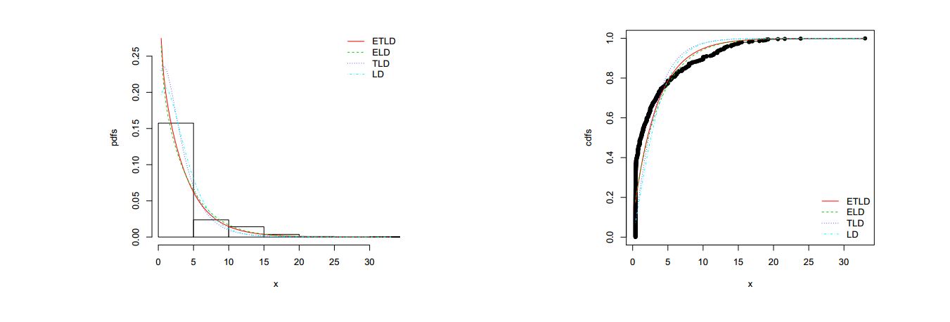
Results in Table 2 indicate that \(ETLD\) corresponds to the smallest AIC and BIC values, making it the best among all the distributions which have been fitted to the data.
Figure 17. Graphs of the estimated pdfs and cdfs based on the first data
For the second data, the maximum likelihood estimates of the model parameters, their respective standard errors and AIC and BIC values are reported in Table 3.
Table 3. Parameter Estimates and Corresponding Values of Model Selection Criteria for the Distributions Fitted to Data 2.
Distribution
Estimate
Standard Error
-LL
AIC
BIC
ETL(\(\alpha,\lambda,\theta\))
\(\hat{\alpha}\)=0.5820
0.0281
1806.964
3619.928
3634.0419
\(\hat{\lambda}\)=0.3918
0.0792
\(\hat{\theta}\)=0.3264
0.0170
EL(\(\alpha,\theta\))
\(\hat{\alpha}\)=0.5396
0.0246
1818.004
3640.008
3649.422
\(\hat{\theta}\)=0.3546
0.0151
TL(\(\lambda,\theta\))
\(\hat{\lambda}\)=0.5022
0.0482
1874.227
3752.453
3761.867
\(\hat{\theta}\)=0.4432
0.0138
L(\(\theta\))
\(\hat{\theta}\)2=0.5099
0.0130
1919.938
3841.876
3846.583
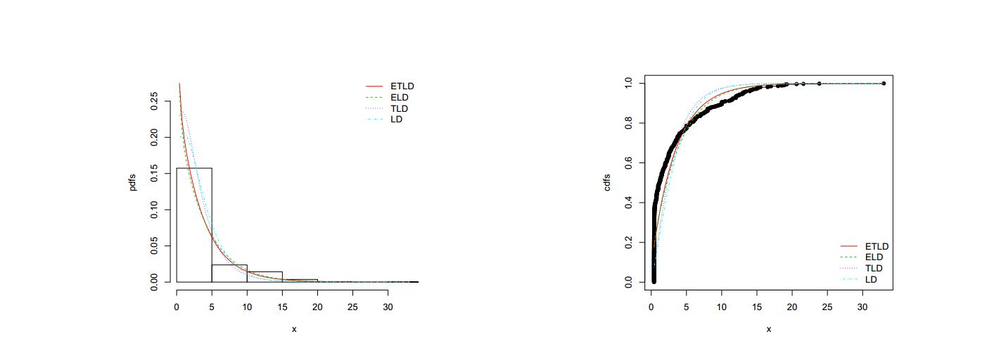
Table 3 clearly shows that the \(ETLD\) has the minimum values of AIC and BIC among the fitted distributions. Thus, the ETL distribution is the best model for modelling the data among the distributions considered in Table 3.
Figure 18. Graphs of the estimated pdfs and cdfs based on the second data
10. Conclusion
In as much as the quality of the empirical results obtained by applying many parametric methods of analysis greatly depends on how well the chosen distribution fits the data under consideration, efforts will always be made to generalize distributions. We have introduced and studied the properties of a new distribution called the exponentiated transmuted Lindley distribution. Specifically,
we have derived the quantile function, the expression for the raw moments, moment generating function and the pdf of the \(kth\) order statistic based on the distribution. Through a numerical illustration, the distribution is found to be capable of being positively skewed and platykurtic or positively skewed and leptokurtic. Under several conditions, the relationships between each of the mean,
median, variance, skewness and kurtosis of the distribution and the parameters are studied. In particular, when only two parameters are constant, it is interesting to know that none of skewness and kurtosis is a linear function of the other parameter. With two data sets, the applicability as well as the ability of this distribution to outperform its sub-models in many data analysis situations is illustrated
. Therefore, the model is recommended for modelling right-skewed data.
Author Contributions
All authors contributed equally to the writing of this paper. All authors read and approved the
final manuscript.
Competing Interests
The author(s) do not have any competing interests in the manuscript.
References
Ghitany, M. E., Atieh, B., & Nadarajah, S. (2008). Lindley distribution and its application. Mathematics and computers in simulation, 78(4), 493-506.[Google Scholor]
Bakouch, H. S., & Popović, B. V. (2016). Lindley first-order autoregressive model with applications. Communications in Statistics-Theory and Methods, 45(17), 4988-5006.[Google Scholor]
Fatima, A., & Roohi, A. (2015). Transmuted exponentiated pareto-i distribution. Pakistan Journal of Statistics, 32(1), 63-80.[Google Scholor]
Nadarajah, S., Bakouch, H. S., & Tahmasbi, R. (2011). A generalized Lindley distribution. Sankhya B, 73(2), 331-359. [Google Scholor]
Merovci, F. (2013). Transmuted lindley distribution. International Journal of Open Problems in Computer Science and Mathematics, 238(1393), 1-20. [Google Scholor]
Mansour, M. M., & Mohamed, S. M. (2015). A new generalized of transmuted Lindley distribution. Appl. Math. Sci, 9, 2729-2748.[Google Scholor]
Kemaloglu, S. A., & Yilmaz, M. (2017). Transmuted two-parameter Lindley distribution. Communications in Statistics-Theory and Methods, 46(23), 11866-11879. [Google Scholor]
Granzotto, D. C., Mazucheli, J., & Louzada, F. (2016). Statistical study of monthly rainfall trends by using the transmuted power Lindley distribution. International Journal of Statistics and Probability, 6(1), 111-124. [Google Scholor]
Nofal, Z. M., & Abd El Hadi, N. E. (2015). Exponentiated transmuted generalized Raleigh distribution: A new four parameter Rayleigh distribution.
Pakistan journal of statistics and operation research, 11(1), 115-134.[Google Scholor]
Fattah, A. A., Nadarajah, S., & Ahmed, A. H. N. (2017). The exponentiated transmuted Weibull geometric distribution with application in survival analysis. Communications in Statistics-Simulation and Computation, 46(6), 4244-4263. [Google Scholor]
Pal, M., & Tiensuwan, M. (2015). Exponentiated transmuted modified Weibull distribution. European Journal of Pure and Applied Mathematics, 8(1), 1-14.[Google Scholor]
Kenney, J. F. (2013). Mathematics of statistics. D. Van Nostrand Company Inc.[Google Scholor]
Moors, J. J. A. (1988). A quantile alternative for kurtosis. Journal of the Royal Statistical Society: Series D (The Statistician), 37(1), 25-32. [Google Scholor]
Smithson, M., & Verkuilen, J. (2006). A better lemon squeezer? Maximum-likelihood regression with beta-distributed dependent variables. Psychological methods, 11(1), 54-71. [Google Scholor]
Bourguignon, M., Ghosh, I., & Cordeiro, G. M. (2016). General results for the transmuted family of distributions and new models. Journal of Probability and Statistics, 2016, 1-12. [Google Scholor]
Oluyede, B. O., & Rajasooriya, S. (2013). The Mc-Dagum distribution and its statistical properties with applications. Asian Journal of Mathematics and Applications, 2013, 1-16.[Google Scholor]