We consider 1D and 2D Schrödinger equation with delta potential on the positive half-axis with Dirichlet, Neumann, and Robin type boundary conditions. We presented and estimated the exact values of the beta critical.
This paper deals with 1D and 2D exactly solvable models for the Schrödinger operators. We study the existence of negative eigenvalues lying
under the continuous spectrum of the Schrödinger operator with \(\delta\) potential.
The main goal is to find the threshold value of the coupling constant for
which such eigenvalues exist. In one dimensional case, our result’s are similar to the consequences of the more general results concerning the Schrödinger operators with a finite number of \(\delta-\)interactions
on the line [1]. In [1], Albeverio and Nizhnik have provided the effective algorithm for determining the number of negative eigenvalues of such operators
in terms of the intensities \(\alpha_k\) and the distances \(d_k = x_{k+1}-x_k\) between the
interactions. In this paper, we consider the eigenvalue problem
on the positive half-axis with Dirichlet, Neumann, and Robin type boundary conditions. For all solvable models under consideration, there exists a critical value \(\beta_{cr}\) such that the operator possesses
the negative eigenvalues if \(\beta>\beta_{cr}\) and has no eigenvalues if \(\beta>\beta_{cr}\). The goal of this paper is to present and estimate the exact values of the beta critical for Eq. (2) considering appropriate boundary condition. We define beta critical as a critical value of the coupling constant denoted by \(\beta_{cr},\) the value of \(\beta\) such that Eq. (2) does not have negative eigenvalues for \(\beta\beta_{cr}\). The delta potential allows solutions for both the bound states \(\lambda 0.\) There has been a considerable interest in the study of coupling constant and the problem was investigated by several researchers like S.Albeverio and others in [2], P.Exner and K.Pankrashkin in [3], Barry Simon in [4], Martin Klaus in [5], and Cranston, Koralov, Molchanov and Vainberg in [7]. It is known that the spectrum of \(-\Delta-\beta V(x)\) consists of the absolutely continuous part \([0, \infty)\) and at most a finite number of of negative eigenvalues
The classification of the spectrum into discrete and continuous parts usually corresponds to a classification of the dynamics into localized (bound) states and locally decaying states when time increases (scattering) respectively. The lower bound, \(0\), of the absolutely continuous spectrum is called the ionization threshold. This follows from the fact that the particle is no longer localized, but moves freely when \(\lambda>0\). This classification is related to the space-time behaviour of solutions of the corresponding Schrödinger equation.
It is known that [7] \(\beta_{cr}>0\) in the case of Dirichlet boundary condition and \(\beta_{cr}=0\) in the case of the Neumann boundary condition in the dimension 1 and 2 . It was shown that the choice \(\beta_{cr}>0\) or \(\beta_{cr}=0\) depends on whether the truncated resolvent is bounded or goes to infinity when \(\lambda\to 0^-\). In fact, \(\beta_{cr}\) was expressed through truncated resolvent operator and depend on the boundary condition and dimension [7]. The main results of this paper in 1D is stated as follows.
Theorem 1.
Consider one dimensional eigenvalue problem
then the \(\beta_{cr}=\frac{1}{a}>0\) in the case of Dirichlet Boundary condition and \(\beta_{cr}=0\) in the case of Neumann and Robin boundary condition.
Proof. The solution of the problem (4) is given by
where \(P\) and \(Q\) are constants and \(\lambda= -k^2 < 0.\)
One can determine the value of constant P and Q by using the Dirichlet condition \(\ y(0)=0\) with \(\ y(a)=1\). Then we split the solution of the problem (4) in to two different regions.
\[
\begin{cases}
y_1(x)= \frac{\sinh kx}{\sinh ka},& \text{if } 0\leq x\leq a\\
y_2(x)= e^{k(a-x)},& \text{if } a\leq x.
\end{cases}
\]
Integrate the Eq. (4) with respect to \(x\) over a small interval \(\Delta \epsilon\) at the point \(x=a\),
\begin{equation}\label{eq6}
\int_{a-\epsilon}^{a+\epsilon}\bigg(-\frac{d^2}{dx^2}-\beta \delta(x-a) y \ \bigg)dx= \int_{a-\epsilon}^{a+\epsilon}(\lambda y)\ dx.
\end{equation}
(6)
The integral of the second derivative is just the first derivative function and the integral over the function in the right hand side goes to zero. This yields,
When \(\epsilon \xrightarrow{}0\), we get
\[ k+k \coth ka =\beta.\]
This implies,
\( \frac{k}{\beta}=\frac{1}{1+ \coth ka}\) and \( \frac{ka}{\beta a}=\frac{1}{1+ \coth ka}\). Let \(ka=A, \ \beta a= B,\) then \(e^{-2A}=1-\frac{2A}{B}.\) Again let \(2A=z, \) then we have,
From Eq. (8), \[1-\frac{z}{B}\geq 0.\]
By solving the inequality, we get \[\frac{\beta}{2}\geq k \] and ultimately,
\(\frac{\beta^2}{4}\geq k^2.\) This leads to
Hence, if \(\beta=0\) then there is no possibility of having negative eigenvalues. Therefore, \(\beta_{cr}\) must be greater than zero to produce negative eigenvalues. We notice that we will not have a solution of the Eq. (8) if \(\frac{1}{B}\geq 1.\) That means, there is no negative eigenvalues when \( \frac{1}{a}\geq \beta. \)
However, for \(\frac{1}{B}\leq 1\), there is a solution of the Eq. (8). That means, when \(\frac{1}{ a}\leq \beta,\) we will have the negative eigenvalues. As we defined \(\beta_{cr},\) the value of \(\beta\) such that Eq. (4) does not have negative eigenvalues for \(\beta\beta_{cr}\), we conclude that \(\beta_{cr}=\frac{1}{a}\) for the Eq. (4) with Dirichlet boundary condition.
If we consider the delta potential located at \(x=a_n\)
then the \(\beta_{cr} \xrightarrow{} \infty \) as \( a_n \xrightarrow{}0.\) That means, if we approach the potential towards to the boundary, i.e., \(a_n \xrightarrow{}0\) then
\(\beta_{cr} \xrightarrow{} \infty .\)
We consider the Neumann boundary condition then the Eq. (2) becomes
Similar to Dirichlet problem, we divide the solution of Neumann problem in to two different regions:
\[
\begin{cases}
y_1(x)= \frac{\cosh kx}{\cosh ka},& \text{if } 0\leq x\leq a\\
y_2(x)= e^{k(a-x)},& \text{if } a\leq x.
\end{cases}
\]
Integrate the Eq. (10) with respect to \(x\) over a small interval and take \(\epsilon \xrightarrow{}0\) yields,
\[ k+k \tanh ka =\beta.\]
After simplification, we get
\[ \frac{k}{\beta}=\frac{1}{1+ \tanh ka} \]
and then we multiply and divide by \(a\) for the right hand side,
\[\frac{ka}{\beta a}=\frac{1}{1+ \tanh ka}.\]
Let \(ka=A,\ \beta a= B\), then \[e^{-2A}=\frac{2A}{B}-1.\]
Following the same analysis as Dirichlet case, we get
\(\frac{\beta^2}{4}\leq k^2.\)
This implies that \(\lambda =-k^2 \leq \frac{-\beta^2}{4}\) and
concludes that if \(\beta=0\) then there is still a possibility of having a negative eigenvalues. Hence, \(\beta_{cr}=0.\)
Now we consider the Robin boundary condition. The Eq. (2) with Robin boundary condition is given by
As above, we divide the solution of this problem in to two different regions:
\[
\begin{cases}
y_1(x)= \frac{k\cosh kx-\sinh kx}{k\cosh ka-\sinh ka},& \text{if } 0\leq x\leq a\\
y_2(x)= e^{k(a-x)},& \text{if } a\leq x.
\end{cases}
\]
We integrate the Eq. (11) with respect to \(x\) over a small interval \(\Delta \epsilon\),
\[\int_{a-\epsilon}^{a+\epsilon}(-y^{”}-\beta \delta(x-a) y \ )dx= \int_{a-\epsilon}^{a+\epsilon}(\lambda y)dx.\]
After integration and taking \( \epsilon \xrightarrow{}0,\) we get,
\[ k+k \bigg(\frac{k-\coth ka}{k\coth ka-1}\bigg) =\beta.\]
After simplification,
\[ \frac{k}{\beta}=\frac{1}{1+ \bigg(\frac{k-\coth ka}{k\coth ka-1}\bigg)} ,\]
and
\[ \frac{ka}{\beta a}=\frac{1}{1+ \bigg(\frac{k-\coth ka}{k\coth ka-1}\bigg)}.\]
Let \(ka=A, \beta a= B\), then \[e^{-2A}=\frac{2A^2-2Aa-AB+Ba}{AB+Ba}.\]
Observe that \(\frac{2A^2-2Aa-AB+Ba}{AB+Ba}\) must be \(\geq 0.\) After solving this inequality, we get \[\frac{\beta}{2}\leq k. \]
Now, \(\lambda =-k^2 \leq \frac{-\beta^2}{4}.\) Hence, if \(\beta=0\) then there is a possibility of having negative eigenvalues so \(\beta_{cr}\) must be zero.
Two Dimensional eigenvalue problem
The rotational invariance suggests that the two dimensional Laplacian should take a particularly simple form in polar coordinates. We use polar coordinates \((r, \theta)\) and look for solutions depending only on r. For \(d=2,\) we do not consider the Neumann boundary condition since \(\beta_{cr}\) is always zero in this case.
Theorem 2.
Consider two dimensional Dirichlet problem with delta potential on the circle,
We divide the solution of Eq. (13) into two different regions: region (I) with \(1\leq r < 1+a\) and region (II) with \(1+a< r\),
\[
\begin{cases}
y_1(r)= \frac{Y_0(k)J_0(kr)-J_0(k)Y_0(kr)}{Y_0(k)J_0(k(1+a))-J_0(k)Y_0(k(1+a))},& \text{if } 1\leq r\leq 1+a\\
y_2(r)= \frac{K_0(kr)}{K_0(k(1+a))},& \text{if } 1+a\leq r.
\end{cases}
\]
Using the same argument as in the one dimensional problem, we get \[ -y^{'}\bigg|_{1+a-\epsilon}^{1+a+\epsilon}-\beta y(1+a)=0.\]
After simplification, we have
\[ -\big(y_2^{'}|_{1+a+\epsilon}-y_1^{'}|_{1+a-\epsilon}\big)=\beta.\]
When \(\epsilon \xrightarrow{}0,\) we get
where \(Y_0\) and \(Y_1\) are Bessel function of second kind and and \(J_0\) and \(J_1\) are Bessel function of first kind. Similarly, \(K_0\) and \(K_1\) are a modified Bessel function of second kind. We define
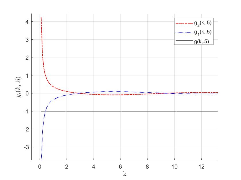
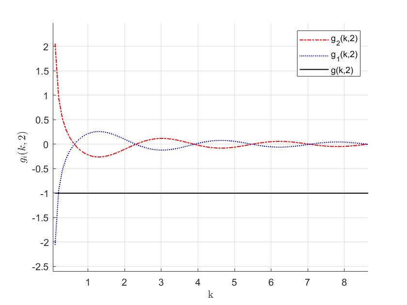
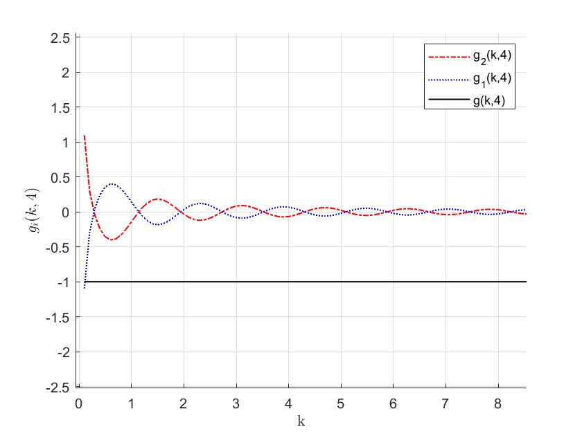
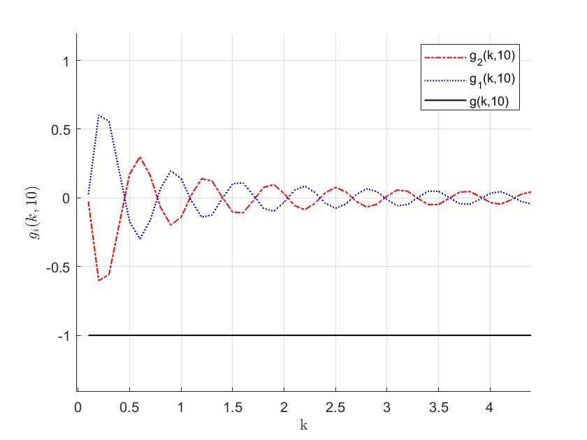
\[ g(k,a)=\frac{g_1(k,a)}{g_2(k,a)}=\frac{-Y_0(k)J_1(k(1+a)+J_0(k)Y_1(k(1+a))}{Y_0(k)J_0(k(1+a))-J_0(k)Y_0(k(1+a))}.\]
We notice that \(g(k,a)=-1\) for all the values of \(a\) as shown in the Figures 1-4.
Figure 1. graph of the function g(k,5).Figure 2. Graph of the function g(k,2).Figure 3. Graph of the function g(k,4).Figure 4. Graph of the function g(k,10).
hold for all \(x>0\) if only if \(p\geq 1/4\) and \(q=0.\)
Now, from Eqs (15) and (16) we get,
\[\frac{1}{2(x+p)}< \frac{K_1(x)}{K_0(x)}-1< \frac{1}{2(x+q)}.\]
When \(x=k(a+1)>0,\)
\[\frac{1}{2(k(a+1)+p)}< \frac{K_1(k(a+1))}{K_0(k(a+1))}-1< \frac{1}{2(k(a+1)+q)}.\]
\[\frac{1}{2(k(a+1)+p)}< \frac{\beta}{k}< \frac{1}{2(k(a+1)+q)}.\]
\[\frac{1}{2((a+1)+\frac{p}{k})}< \beta < \frac{1}{2((a+1)+\frac{q}{k})}.\]
Since \(a>0, p\geq \frac{1}{4}, k>0\), which tells us that \(\beta >0\) and hence \(\beta_{cr}>0\) and \(\beta \in (0,\frac{1}{2}).\)
Conflicts of Interest:
The author declares no conflict of interest.
Data Availability:
All data required for this research is included within this paper.
Funding Information:
No funding is available for this research.
References
Albeverio, S., & Nizhnik, L. (2003). On the number of negative eigenvalues of a one-dimensional Schrödinger operator with point interactions. Letters in Mathematical Physics, 65(1), 27-35. [Google Scholor]
Albeverio, S., Gesztesy, F., Hoegh-Krohn, R., & Holden, H. (2012). Solvable Models in Quantum Mechanics. Springer Science & Business Media. [Google Scholor]
Exner, P., & Pankrashkin, K. (2014). Strong coupling asymptotics for a singular Schrödinger operator with an interaction supported by an open arc. Communications in Partial Differential Equations, 39(2), 193-212. [Google Scholor]
Simon, B. (1976). The bound state of weakly coupled Schrödinger operators in one and two dimensions. Annals of Physics, 97(2), 279-288. [Google Scholor]
Klaus, M. (1977). On the bound state of Schrödinger operators in one dimension. Annals of Physics, 108(2), 288-300.[Google Scholor]
Cranston, M., Koralov, L., Molchanov, S., & Vainberg, B. (2009). Continuous model for homopolymers. Journal of Functional Analysis, 256(8), 2656-2696. [Google Scholor]
Puri, R., & Vainberg, B. (2022). On the critical value of the coupling constant in exterior elliptic problems. Applicable Analysis, 101(1), 108-117. [Google Scholor]
Yang, Z. H., & Chu, Y. M. (2017). On approximating the modified Bessel function of the second kind. Journal of Inequalities and Applications, 2017, Article No 47. https://doi.org/10.1186/s13660-017-1317-z.[Google Scholor]