Open Journal of Mathematical Sciences

On Unsteady Flow of a Viscoelastic Fluid Through Rotating Cylinders

Madeeha Tahir\(^1\), Muhammad Nawaz Naeem, Rabia Safdar, Dumitru Vieru, Muhammad Imran
Department of Mathematics, Government College University, Faisalabad, Pakistan. (M.T & M.N.N & R.S & M.I)
Department of Theoretical Mechanics Technical University Gh. Asachi Iasi Romania. (D.V)
\(^1\) Corresponding Author;  dr.madeeha.2017@gmail.com
Copyright © 2017 Madeeha Tahir, Muhammad Nawaz Naeem, Rabia Safdar, Dumitru Vieru, Muhammad Imran. This is an open access article distributed under the Creative Commons Attribution License, which permits unrestricted use, distribution, and reproduction in any medium, provided the original work is properly cited.

Abstract

The fractional calculus approach is used in the constitutive relationship model of fractional Maxwell fluid. Exact solutions for the velocity field and the adequate shear stress corresponding to the rotational flow of a fractional Maxwell fluid, between two infinite coaxial circular cylinders, are obtained by using the Laplace transform and finite Hankel transform for fractional calculus. The solutions that have been obtained are presented in terms of generalized \(G_{b, c, d}(\cdot, t)\) and \(R_{b, c}(\cdot, t)\) functions. In the limiting cases, the corresponding solutions for ordinary Maxwell and Newtonian fluids are obtained from our general solutions. Furthermore, the solutions for the motion between the cylinders, when one of them is at rest, are also obtained as special cases from our results. Finally, the influence of the material parameters on the fluid motion is underlined by graphical illustrations.

Keywords:

Fractional Maxwell fluid, Coaxial cylinders, Unsteady rotating flow, Velocity field, Shear stress. Laplace and finite Hankel transforms.

1. Introduction

All things are movable and in a fluid state, which is a famous quotation from Thales of Miletos, the first philosopher of Ancient Greece.
The inadequacy of the classical Navier–Stokes theory to describe rheologically complex fluids such as polymer solutions, blood and heavy oils, has led to the development of theories of non-Newtonian fluids. In particular many pastes, slurries, synovial polymer solutions and suspensions exhibit shear thinning behavior. In recent time the study of non-Newtonian fluids has become important. Chemical engineering, food industry, biological analysis, petroleum industry and many other fields use them. The academic workers and engineers are very much interested in the geometry of flows of such types of fluids [1, 2]. In order to describe the non-linear relationship between the stress and the strain rate, numerous models or constitutive equations have been proposed. Models of differential type and rate type have received much attention [3].
In recent years, the fractional Maxwell fluid has obtained a special attention amongst many fluids of rate type, as it includes as special cases the classical Newtonian fluid and the ordinary Maxwell fluid. Fractional calculus has encountered much success in the description of viscoelastic characteristics. The starting point of the fractional derivative model of non-Newtonian model is usually a classical differential equation which is modified by replacing the time derivative of an integer order by the so-called Caputo fractional calculus operator. This generalization allows one to define precisely non-integer order integrals or derivatives [4]. Fractional calculus has been found to be quite flexible in describing viscoelastic behavior [5, 6, 7].
During the past few years, attention has been given to the study on rotating flow of viscoelastic fluids in an annulus. In those studies, the Maxwell model was adopted to describe the viscoelastic fluid. The unidirectional flow of viscoelastic fluid with the fractional Maxwell model was studied by Tan et al. [8, 9] and Hayat et al. [10]. Qi et al. [11, 12] studied the unsteady flow of a viscoelastic fluid with fractional Maxwell model. Recently, Fetecau et al. [13] and Mahmood et al. [14] also studied the flow of fractional Maxwell fluid between coaxial cylinders. There is a vast literature dealing with such fluids, but we shall recall here only a few of the recent papers [15, 16, 17, 18, 19, 20, 21, 22, 23, 24, 25,26 ] in cylindrical domains.
The aim of this paper is to establish exact solutions of the velocity field and the shear stress corresponding to the motion of a fractional Maxwell fluid between two infinite circular cylinders. The laplace and finite Hankel transforms are used to solve the problem and the solutions obtained are presented in terms of generalized \(G_{b, c, d}(\cdot, t)\) and \(R_{b, c}(\cdot, t)\) functions. The solutions for ordinary Maxwell and Newtonian fluids are obtained as limiting cases of our general solutions. Furthermore, the solutions for the motion between the cylinders, when one of them is at rest, are also obtained as special cases from our general results. Finally, the influence of the material parameters on the velocity and shear stress of the fluid is analyzed by graphical illustrations.

2. Formulation of the Problem

For the problem under consideration, we choose the cylindrical coordinates \((r, \theta, z)\) and the components of velocity field \(\textbf{w}(r, t)\) are \(w_{r}=0\), \(w_{\theta}=w(r, t)\), \(w_{z}=0\). Since the velocity field \(\textbf{w}\) is independent of \(\theta\) and \(z\), we also assume that the extra-stress tensor \(\textbf{S}\) depends only on \(r\) and \(t\). Furthermore, if the fluid is assumed to be at rest at the moment \(t = 0\), then
\begin{align}\label{Bellman-eq01} \textbf{w}(r,0)=\textbf{0},\,\,\,\,\,\,\textbf{S}(r,0)=\textbf{0}. \end{align}
(1)
For an incompressible fluid, the equation of continuity is
\begin{align}\label{Bellman-eq04} \nabla\cdot\textbf{w}=0, \end{align}
(2)
and in the absence of body forces and pressure gradient, the equation of motion is
\begin{align}\label{Bellman-eq05} \rho\frac{D\textbf{w}}{Dt}=\nabla\cdot \textbf{T}, \end{align}
(3)
where \(\rho\) is the density of the fluid, \(D/Dt\) is the material derivative and \(\textbf{T}\) is the stress tensor. According to the above conditions, the constitutive equation and the equation of motion become [11]
\begin{align}\label{Bellman-eq06} \tau(r,t)+\lambda^{\alpha}D_{t}^{\alpha}\tau(r,t)=\mu r\frac{\partial}{\partial r}\left(\frac{w(r, t)}{r}\right), \end{align}
(4)
and respectively
\begin{align}\label{Bellman-eq07} \rho \frac{\partial w(r, t)}{\partial t}=\frac{1}{r^{2}}\frac{\partial}{\partial r}(r^{2}\tau(r,t)). \end{align}
(5)
Eliminating \(\tau(r,t)\) from Eqs. (4) and (5), we obtain the governing equation of the fluid
\begin{align}\label{Bellman-eq08} (1+\lambda D^\alpha_{t})\frac{\partial w(r, t)}{\partial t}= \nu \left(\frac{\partial^2} {\partial r^2}+\frac{1}{r}\frac{\partial}{\partial r}-\frac{1}{r^{2}}\right)w(r, t), \end{align}
(6)
where \(\nu=\mu/\rho\) is the kinematic viscosity of the fluid.
We consider an incompressible fractional Maxwell fluid at rest in an annular region between two coaxial circular cylinders of radii \(R_1\) and \(R_2(>R_1)\). At time \(t=0^{+}\), both cylinders begin to rotate along their common axis. It is obvious that the motion between the two cylinders is axially symmetric. Owing to the shear, the fluid is gradually moved with the appropriate initial and boundary conditions
\begin{align}\label{Bellman-eq09} w(r,0)=\frac{\partial w(r,0)}{\partial t}=0\,,\,\,\tau(r,0)=0;\,\,\,\,\,\,\,\,r\in[R_1,R_2], \end{align}
(7)
\begin{align}\label{Bellman-eq10} w(R_1,t)=\Omega_{1}R_{1}t^{a},\,\,\,\,w(R_2,t)=\Omega_{2}R_{2}t^{a}\,\,\,\,\textrm{for}\,\,\,t\geq 0\,\,\,\,\,a>0, \end{align}
(8)
where \(\Omega_{1}\) and \(\Omega_{2}\) are constants.

3. Solution of the Problem

In order to solve the problem Eqs. (4) and (6) with initial and boundary conditions (7) and (8), we shall use the Laplace and the Hankel transforms. Laplace transform is used to eliminate the time variable and to eliminate spatial variable, Hankel transform is used. To avoid from lengthy calculations of residues and contours integrals, the discrete inverse Laplace method will be used.

3.1. Calculation of the Velocity Field

Applying the Laplace transform to Eqs. (6) and (8), using (7) and formulae
\begin{align}\label{Bellman-eq11} L\left\{D_{t}^{\beta}f(t)\right\}=q^{\beta}L\left\{f(t)\right\},\,\,\,\,\, L\left\{t^{n}\right\}=\frac{\Gamma(n+1)}{q^{n+1}};\,\,\,n>-1, \end{align}
(9)
we find that
\begin{align}\label{Bellman-eq12} (q+\lambda q^{\alpha+1})\overline{w}(r,q)=\nu\left(\frac{\partial^2} {\partial r^2}+\frac{1}{r}\frac{\partial}{\partial r}-\frac{1}{r^{2}}\right)\overline{w}(r,q) ;\,\,\,\,\,\,\,\,\,\,\,\,\,\,\,\,\,r\in[R_1,R_2], \end{align}
(10)
\begin{align}\label{Bellman-eq13} \overline{w}(R_1,q)=\frac{\Omega_{1}R_{1}\Gamma(a+1)}{q^{a+1}},\,\,\,\,\overline{w}(R_2,q) =\frac{\Omega_{2}R_{2}\Gamma(a+1)}{q^{a+1}}, \end{align}
(11)
where \(\overline{w}(r,q)=\int_{0}^{\infty}w(r,t)e^{-qt}dt\) is the Laplace transform of \(w(r,t)\) and \(q\) is the transform parameter.
The Hankel transform of \(\overline{w}(r,q)\) is defined as
\begin{align}\label{Bellman-eq14} \overline{w}_{H}(r_{n},q)=\int_{R_1}^{R_2} r\overline{w}(r,q)B(r, r_{n})dr, \end{align}
(12)
where
\begin{align}\label{Bellman-eq15} B(r, r_{n})=J_{1}(rr_{n})Y_{1}(R_{2}r_{n})-J_{1}(R_{2}r_{n})Y_{1}(rr_{n}), \end{align}
(13)
here \(r_{n}\) are the positive roots of the transcendental equation \(B(R_{1}, r)=0 \) while \(J_{1}(\cdot)\) and \(Y_{1}(\cdot)\) are the first and second kind Bessel functions of 1st order.
Now, applying the Hankel transform to Eq. (9), taking into account the conditions (10) and the identity
\begin{align}\label{Bellman-eq16} &\int_{R_1}^{R_2}\!\!\!r\left\{\frac{\partial^2}{\partial r^2}+\frac{1}{r} \frac{\partial}{\partial r}-\frac{1}{r^{2}}\right\}\overline{w}(r,q)B(r, r_{n})dr \nonumber\\&= \frac{2}{\pi q^{2}} \left\{\frac{\Omega_{2}R_{2}J_{1}(R_{1}r_{n})-\Omega_{1}R_{1}J_{1}(R_{2}r_{n})}{J_{1}(R_{1}r_{n})}\right\} - r_{n}^{2}\overline{w}_{H}(r_{n},q), \end{align}
(14)
we find that
\begin{align}\label{Bellman-eq17} \overline{w}_{H}(r_{n},q)=\frac{2\nu \left\{\Omega_{2}R_{2}J_{1}(R_{1}r_{n})-\Omega_{1}R_{1} J_{1}(R_{2}r_{n})\right\}\Gamma(a+1)}{\pi J_{1}(R_{1}r_{n})\,q^{a+1}(\lambda q^{\alpha+1}+q+\nu r_{n}^{2})}. \end{align}
(15)
In order to obtain the velocity field \(w(r, t)\), we have to apply the inverse transforms (both laplace and Hankel). For this, the above Eq. (14) can be written as
\begin{align}\label{Bellman-eq18} \overline{w}_{H}(r_{n},q)&=\frac{2\left\{\Omega_{2}R_{2}J_{1}(R_{1}r_{n})-\Omega_{1}R_{1}J_{1}(R_{2}r_{n})\right\} \Gamma(a+1)}{\pi r_{n}^{2} J_{1}(R_{1}r_{n})} \nonumber \\ &\times\left\{\frac{1}{q^{a+1}}-\frac{1+\lambda q^{\alpha}}{q^{a}\left(\lambda q^{\alpha+1}+q+\nu r_{n}^{2}\right)}\right\}. \end{align}
(16)
Using the formula [27]
\begin{align}\label{Bellman-eq19} \overline{w}(r,q)=\frac{\pi^{2}}{2}\sum_{n=1}^{\infty}\frac{r_{n}^{2}J_{1}^{2}(R_{1}r_{n})B(r, r_{n})} {J_{1}^{2}(R_{1}r_{n})-J_{1}^{2}(R_{2}r_{n})}\,\overline{w}_{H}(r_{n},q), \end{align}
(17)
the inverse Hankel transform of \(\overline{w}_{H}(r_{n},q)\) is given as
\begin{align}\label{Bellman-eq20} \overline{w}(r,q)=&\frac{\Omega_{1}R_{1}^{2}(R_{2}^{2}-r^{2})+\Omega_{2}R_{2}^{2}(r^{2}-R_{1}^{2})} {r(R_{2}^{2}-R_{1}^{2})}\frac{\Gamma(a+1)}{q^{a+1}}-\pi \Gamma(a+1)\nonumber\\&\times \sum_{n=1}^{\infty}\frac{J_{1}(R_{1}r_{n})B(r, r_{n})}{J_{1}^{2}(R_{1}r_{n})-J_{1}^{2}(R_{2}r_{n})} \left\{\Omega_{2}R_{2}J_{1}(R_{1}r_{n})-\Omega_{1}R_{1}J_{1}(R_{2}r_{n})\right\} \nonumber\\&\times \frac{1+\lambda q^{\alpha}}{q^{a}\left(\lambda q^{\alpha+1}+q+\nu r_{n}^{2}\right)}. \end{align}
(18)
Finally, using the expansion
\begin{align}\label{Bellman-eq21} \frac{1+\lambda q^{\alpha}}{q^{a}\left(\lambda q^{\alpha+1}+q+\nu r_{n}^{2}\right)}=\frac{1}{\lambda}\sum_{k=0}^\infty \left(\frac{-\nu r_n^2}{\lambda}\right)^{k}\left[\frac{q^{-a-k-1}}{(q^{\alpha}+\lambda^{-1})^{k+1}}+ \frac{\lambda \,q^{\alpha-a-k-1}}{(q^{\alpha}+\lambda^{-1})^{k+1}}\right], \end{align}
(19)
and the known formulae [28]
\begin{equation}\label{Bellman-eq22} L^{-1}\bigg\{\frac{1}{q^{f}}\bigg\}=\frac{t^{f-1}}{\Gamma(f)}\,,\,\,\,f>0\,, \end{equation}
(20)
\begin{equation}\label{Bellman-eq23} L^{-1}\bigg\{\frac{q^{c}}{(q^{b}-p)^{d}}\bigg\}=G_{b,\,c,\,d}(p,t)\,,\,\,\,Re(bd-c)>0, \,\,\,\,\,|\frac{p}{q^{b}}|< 1\,, \end{equation}
(21)
where the generalized \(G_{b,\, c,\, d}(\cdot, \cdot)\) function is defined by Eqs. (97) and (101) of [28]
\begin{align}\label{Bellman-eq24} G_{b,\, c,\, d}(p,\, t)=\sum_{j=0}^\infty\frac{p^j \Gamma(d + j)}{\Gamma(d)\Gamma(j + 1)}\frac{t^{(d+j)b-c-1}}{\Gamma[(d+j)b-c]}, \end{align}
(22)
and applying the discrete inverse Laplace transform to Eq. (17), we obtain the velocity field \(w(r, t)\) under the form
\begin{align}\label{Bellman-eq25} w(r,t) &= \frac{\Omega_{1}R_{1}^{2}(R_{2}^{2}-r^{2})+\Omega_{2}R_{2}^{2}(r^{2}-R_{1}^{2})}{r(R_{2}^{2}-R_{1}^{2})} t^{a}-\frac{\pi \Gamma(a+1)}{\lambda} \nonumber\\&\times\sum_{n=1}^{\infty}\frac{J_{1}(R_{1}r_{n})B(r, r_{n})\left\{\Omega_{2}R_{2}J_{1}(R_{1}r_{n})- \Omega_{1}R_{1}J_{1}(R_{2}r_{n})\right\}}{J_{1}^{2}(R_{1}r_{n})-J_{1}^{2}(R_{2}r_{n})} \sum_{k=0}^\infty \left(\frac{-\nu r_n^2}{\lambda}\right)^{k}\nonumber\\ &\times \left\{G_{\alpha,-a-k-1,k+1}\left(-\lambda^{-1},t\right)+\lambda G_{\alpha,\, \alpha-a-k-1,k+1}\left(-\lambda^{-1},t\right)\right\}. \end{align}
(23)

3.2. Calculation of the Shear Stress

Applying the Laplace transform to Eq. (4) and using the condition \((7)_{3}\), we find that
\begin{align}\label{Bellman-eq26} \overline{\tau}(r,q)=\frac{\mu}{1+\lambda q^{\alpha}}\left(\frac{\partial \overline{w}(r,q)}{\partial r}-\frac{\overline{w}(r,q)}{ r}\right), \end{align}
(24)
where
\begin{align}\label{Bellman-eq27} &\frac{\partial \overline{w}(r,q)}{\partial r}-\frac{\overline{w}(r,q)}{ r}=\frac{2R_{1}^{2}R_{2}^{2} (\Omega_{2}-\Omega_{1})}{r^{2}(R_{2}^{2}-R_{1}^{2})}\frac{\Gamma(a+1)}{q^{a+1}}+\pi\Gamma(a+1)\nonumber\\ &\times \sum_{n=1}^{\infty}\frac{J_{1}(R_{1}r_{n})\left(\frac{2}{r}B(r, r_{n})-r_{n}\widetilde{B}(r,r_{n})\right)} {J_{1}^{2}(R_{1}r_{n})-J_{1}^{2}(R_{2}r_{n})}\left\{\Omega_{2}R_{2}J_{1}(R_{1}r_{n})- \Omega_{1}R_{1}J_{1}(R_{2}r_{n})\right\} \nonumber\\ &\times\frac{1+\lambda q^{\alpha}} {q^{a}\left(\lambda q^{\alpha+1}+q+\nu r_{n}^{2}\right)}. \end{align}
(25)
is obtained from Eq. (18) and \begin{align*} \widetilde{B}(rr_{n})=J_{0}(rr_{n})Y_{1}(R_{2}r_{n})-J_{1}(R_{2}r_{n})Y_{0}(rr_{n}). \end{align*} Thus Eq. (24) becomes
\begin{align}\label{Bellman-eq28} \overline{\tau}(r,q)&=\frac{2\mu R_{1}^{2}R_{2}^{2}(\Omega_{2}-\Omega_{1})}{r^{2} (R_{2}^{2}-R_{1}^{2})}\frac{\Gamma(a+1)}{q^{a+1}(1+\lambda q^{\alpha})}+\nonumber\\+&\pi\mu\Gamma(a+1)\sum_{n=1}^{\infty}\frac{J_{1}(R_{1}r_{n})\left(\frac{2}{r} B(r, r_{n})-r_{n}\widetilde{B}(r,r_{n})\right)}{J_{1}^{2}(R_{1}r_{n})-J_{1}^{2}(R_{2}r_{n})}\times \nonumber\\ \times&\left\{\Omega_{2}R_{2}J_{1}(R_{1}r_{n})-\Omega_{1}R_{1}J_{1}(R_{2}r_{n})\right\} \frac{1}{q^{a}\left(\lambda q^{\alpha+1}+q+\nu r_{n}^{2}\right)}, \end{align}
(26)
applying again the discrete inverse Laplace transform as well as using the known relation [28]
\begin{align}\label{Bellman-eq29} \mathcal{L}^{-1}\bigg\{\frac{q^{c}}{q^{b}-d}\bigg\}=R_{b, c}(d,t);\,\,\,\,\mbox{Re}\left(b-c\right)>0,\,\,\,\,\mbox{Re}(q)>0, \end{align}
(27)
where the generalized \(R_{b, c}(d,t)\) functions are defined by [28]
\begin{align}\label{Bellman-eq30} R_{b, c}(d,t)=\sum_{n=0}^\infty\frac{d^{n} t^{(n+1)b-c-1}}{\Gamma[(n+1)b-c]} \end{align}
(28)
and the expansion
\begin{align}\label{Bellman-eq31} \frac{1}{q^{a}\left(\lambda q^{\alpha+1}+q+\nu r_{n}^{2}\right)}=\frac{1}{\lambda}\sum_{k=0}^\infty \left(\frac{-\nu r_n^2}{\lambda}\right)^{k}\frac{q^{-a-k-1}}{(q^{\alpha}+\lambda^{-1})^{k+1}}, \end{align}
(29)
we obtain the shear stress \(\tau(r, t)\) under the form
\begin{align}\label{Bellman-eq32} \tau(r,t)&=\frac{2\mu R_{1}^{2}R_{2}^{2}(\Omega_{2}-\Omega_{1})}{\lambda r^{2}(R_{2}^{2} -R_{1}^{2})}R_{\alpha, -a-1}\left(-\lambda^{-1}, t\right)+\frac{\pi\mu \Gamma(a+1)} {\lambda}\nonumber\\&\times\sum_{n=1}^{\infty}\frac{J_{1}(R_{1}r_{n})\left(\frac{2}{r}B(r, r_{n})-r_{n}\widetilde{B}(r,r_{n}) \right)}{J_{1}^{2}(R_{1}r_{n})-J_{1}^{2}(R_{2}r_{n})}\{\Omega_{2} R_{2}J_{1}(R_{1}r_{n})\nonumber\\&-\Omega_{1}R_{1}J_{1}(R_{2}r_{n})\} \sum_{k=0}^\infty \left(\frac{-\nu r_n^2}{\lambda}\right)^{k}G_{\alpha,-a-k-1,k+1}\left(-\lambda^{-1},t\right). \end{align}
(30)

4. Limiting cases

Case I: Making \(\alpha\rightarrow 1\) into Eqs. (23) and (30), we obtain the velocity field
\begin{align}\label{Bellman-eq33} w_{{}_M}(r,t)&=\frac{\Omega_{1}R_{1}^{2}(R_{2}^{2}-r^{2})+\Omega_{2}R_{2}^{2}(r^{2}-R_{1}^{2})}{r(R_{2}^{2} -R_{1}^{2})} t^{a}-\frac{\pi \Gamma(a+1)}{\lambda} \nonumber\\&\times\sum_{n=1}^{\infty}\frac{J_{1}(R_{1}r_{n})B(r, r_{n})}{J_{1}^{2}(R_{1}r_{n})-J_{1}^{2}(R_{2}r_{n})}\left\{\Omega_{2}R_{2}J_{1}(R_{1}r_{n})- \Omega_{1}R_{1}J_{1}(R_{2}r_{n})\right\}\times \nonumber\\&\times \sum_{k=0}^\infty \left(\frac{-\nu r_n^2}{\lambda}\right)^{k}\left\{G_{1,-a-k-1,k+1}\left(-\lambda^{-1},t\right)+\lambda G_{1,\, -a-k,k+1}\left(-\lambda^{-1},t\right)\right\}. \end{align}
(31)
and the shear stress
\begin{align}\label{Bellman-eq34} \tau_{{}_M}(r,t)&=\frac{2\mu R_{1}^{2}R_{2}^{2}(\Omega_{2}-\Omega_{1})}{\lambda r^{2}(R_{2}^{2}-R_{1}^{2})}R_{1, -a-1}\left(-\lambda^{-1}, t\right)+\nonumber\\&\frac{\pi\mu \Gamma(a+1)}{\lambda}\sum_{n=1}^{\infty}\frac{J_{1}(R_{1}r_{n})\left(\frac{2}{r}B(r, r_{n})-r_{n} \widetilde{B}(r,r_{n})\right)}{J_{1}^{2}(R_{1}r_{n})-J_{1}^{2}(R_{2}r_{n})} \{\Omega_{2}R_{2}J_{1}(R_{1}r_{n})\nonumber\\&-\Omega_{1}R_{1}J_{1}(R_{2}r_{n})\}\sum_{k=0}^\infty \left(\frac{-\nu r_n^2}{\lambda}\right)^{k}G_{1,-a-k-1,k+1}\left(-\lambda^{-1},t\right) \end{align}
(32)
corresponding to an ordinary Maxwell fluid, performing the same motion.
Case II: By now letting \(\lambda\rightarrow 0\) into Eqs. (31) and (32) or \(\alpha\rightarrow 1\) and \(\lambda\rightarrow 0\) into Eqs. (23) and (30), using \(\mathop{\lim}\limits_{\lambda\to 0} \frac{1}{\lambda^{k}}G_{1,\,b,\,k}\left(-\lambda^{-1}, t\right)=\frac{t^{-b-1}}{\Gamma(-b)};\,\,\,b< 0\), we obtain the velocity field
\begin{align}\label{Bellman-eq35} w_{_N}(r,t)=&\frac{\Omega_{1}R_{1}^{2}(R_{2}^{2}-r^{2})+\Omega_{2}R_{2}^{2} (r^{2}-R_{1}^{2})}{r(R_{2}^{2} -R_{1}^{2})} t^{a}-\pi \Gamma(a+1)\nonumber\\ \times& \sum_{n=1}^{\infty}\frac{J_{1}(R_{1}r_{n})B(r, r_{n})}{J_{1}^{2}(R_{1}r_{n})-J_{1}^{2}(R_{2}r_{n})} \left\{\Omega_{2}R_{2}J_{1}(R_{1}r_{n})- \Omega_{1}R_{1}J_{1}(R_{2}r_{n})\right\} \nonumber\\ \times&\sum_{k=0}^\infty \left(-\nu r_n^2\right)^{k}\frac{t^{a+k}}{\Gamma(a+k+1)}, \end{align}
(33)
and the associated shear stress
\begin{align}\label{Bellman-eq36} \tau_{{}_N}(r,t)=&\frac{2\mu R_{1}^{2}R_{2}^{2}(\Omega_{2}-\Omega_{1})}{\lambda r^{2}(R_{2}^{2}-R_{1}^{2})}R_{1, -a-1}\left(-\lambda^{-1}, t\right)+\nonumber\\+&\pi\mu \Gamma(a+1)\sum_{n=1}^{\infty}\frac{J_{1}(R_{1}r_{n})\left(\frac{2}{r}B(r, r_{n})-r_{n} \widetilde{B}(r,r_{n})\right)}{J_{1}^{2}(R_{1}r_{n})-J_{1}^{2}(R_{2}r_{n})}\times\nonumber\\\times & \left\{\Omega_{2}R_{2}J_{1}(R_{1}r_{n})-\Omega_{1}R_{1}J_{1}(R_{2}r_{n})\right\}\sum_{k=0}^\infty \left(-\nu r_n^2\right)^{k}\frac{t^{a+k}}{\Gamma(a+k+1)} \end{align}
(34)
corresponding to a Newtonian fluid, performing the same motion.

5. Special cases

Making \(a=1\) in Eqs. (23) and (30), the solution for the velocity field
\begin{align}\label{Bellman-eq37} w_{{}_1}(r,t) &= \frac{\Omega_{1}R_{1}^{2}(R_{2}^{2}-r^{2})+\Omega_{2}R_{2}^{2}(r^{2}-R_{1}^{2})}{r(R_{2}^{2}-R_{1}^{2})} t-\nonumber\\-&\frac{\pi}{\lambda} \sum_{n=1}^{\infty}\frac{J_{1}(R_{1}r_{n})B(r, r_{n})}{J_{1}^{2}(R_{1}r_{n})-J_{1}^{2}(R_{2}r_{n})}\left\{\Omega_{2}R_{2}J_{1}(R_{1}r_{n})- \Omega_{1}R_{1}J_{1}(R_{2}r_{n})\right\}\times \nonumber\\&\times \sum_{k=0}^\infty \left(\frac{-\nu r_n^2}{\lambda}\right)^{k}\left\{G_{\alpha,-k-2,k+1}\left(-\lambda^{-1},t\right)+\lambda G_{\alpha,\, \alpha-k-2,k+1}\left(-\lambda^{-1},t\right)\right\}. \end{align}
(35)
and the shear stress
\begin{align}\label{Bellman-eq38} \tau_{{}_1}(r,t)=&\frac{2\mu R_{1}^{2}R_{2}^{2}(\Omega_{2}-\Omega_{1})}{\lambda r^{2}(R_{2}^{2} -R_{1}^{2})}R_{\alpha, -2}\left(-\lambda^{-1}, t\right)+\nonumber\\+&\frac{\pi\mu} {\lambda}\sum_{n=1}^{\infty}\frac{J_{1}(R_{1}r_{n})\left(\frac{2}{r}B(r, r_{n})-r_{n}\widetilde{B}(r,r_{n}) \right)}{J_{1}^{2}(R_{1}r_{n})-J_{1}^{2}(R_{2}r_{n})}\{\Omega_{2} R_{2}J_{1}(R_{1}r_{n}) \nonumber\\ &-\Omega_{1}R_{1}J_{1}(R_{2}r_{n})\}\sum_{k=0}^\infty \left(\frac{-\nu r_n^2}{\lambda}\right)^{k}G_{\alpha,-k-2,k+1}\left(-\lambda^{-1},t\right) \end{align}
(36)
are recovered which are identical to [26].
Now making again \(a=0\) in Eqs. (24) and (32), the solutions
\begin{align}\label{Bellman-eq39} w_{{}_{1M}}(r,t)&=\frac{\Omega_{1}R_{1}^{2}(R_{2}^{2}-r^{2})+\Omega_{2}R_{2}^{2}(r^{2}-R_{1}^{2})} {r(R_{2}^{2}-R_{1}^{2})} t-\nonumber\\&-\frac{\pi}{\lambda} \sum_{n=1}^{\infty}\frac{J_{1} (R_{1}r_{n})B(r, r_{n})}{J_{1}^{2}(R_{1}r_{n})-J_{1}^{2}(R_{2}r_{n})}\left\{\Omega_{2}R_{2}J_{1}(R_{1}r_{n})- \Omega_{1}R_{1}J_{1}(R_{2}r_{n})\right\}\times \nonumber\\&\times \sum_{k=0}^\infty \left(\frac{-\nu r_n^2}{\lambda}\right)^{k}\left\{G_{1,-k-2,k+1}\left(-\lambda^{-1},t\right)+\lambda G_{1,\, -k-1,k+1}\left(-\lambda^{-1},t\right)\right\}\nonumber\\ &=\frac{\Omega_{1}R_{1}^{2}(R_{2}^{2}-r^{2})+\Omega_{2}R_{2}^{2}(r^{2}-R_{1}^{2})} {r(R_{2}^{2}-R_{1}^{2})} t -\frac{\pi}{\nu} \sum_{n=1}^{\infty}\frac{J_{1}(R_{1}r_{n})B(r, r_{n})}{r_{n}^{2}[J_{1}^{2}(R_{1}r_{n})-J_{1}^{2}(R_{2}r_{n})]} \nonumber\\&\times\left\{\Omega_{2}R_{2}J_{1}(R_{1}r_{n})- \Omega_{1}R_{1}J_{1}(R_{2}r_{n})\right\} \left\{1- \lambda\frac{q_{1n}^{2}e^{q_{2n} t}-q_{2n}^{2}e^{q_{1n} t}}{q_{2n}-q_{1n}}\right\}\,, \end{align}
(37)
and the shear stress
\begin{align}\label{Bellman-eq40} \tau_{{}_{1M}}(r,t)&=\frac{2\mu R_{1}^{2}R_{2}^{2}(\Omega_{2}-\Omega_{1})}{\lambda r^{2}(R_{2}^{2}-R_{1}^{2})}R_{1, -2}\left(-\lambda^{-1}, t\right)+\frac{\pi\mu} {\lambda}\nonumber\\&\times\sum_{n=1}^{\infty}\frac{J_{1}(R_{1}r_{n})\left(\frac{2}{r}B(r, r_{n})-r_{n} \widetilde{B}(r,r_{n})\right)}{J_{1}^{2}(R_{1}r_{n})-J_{1}^{2}(R_{2}r_{n})} \{\Omega_{2}R_{2}J_{1}(R_{1}r_{n})\nonumber\\&- \Omega_{1}R_{1}J_{1}(R_{2}r_{n})\}\sum_{k=0}^\infty \left(\frac{-\nu r_n^2}{\lambda}\right)^{k}G_{1,-k-2,k+1}\left(-\lambda^{-1},t\right)\nonumber\\ &=\frac{2\mu R_{1}^{2}R_{2}^{2}(\Omega_{2}-\Omega_{1})}{ r^{2}(R_{2}^{2}-R_{1}^{2})} \left\{t-\lambda\left(1-e^{-t/\lambda}\right)\right\}+\pi\rho\nonumber\\&\times\sum_{n=1}^{\infty} \frac{J_{1}(R_{1}r_{n})\left(\frac{2}{r}B(r, r_{n})-r_{n}\widetilde{B}(r,r_{n})\right)} {r_{n}^{2}[J_{1}^{2}(R_{1}r_{n})-J_{1}^{2}(R_{2}r_{n})]}\{\Omega_{2}R_{2} J_{1}(R_{1}r_{n})\nonumber\\&-\Omega_{1}R_{1}J_{1}(R_{2}r_{n})\}\left\{1+\frac{q_{1n}e^{q_{2n} t}-q_{2n}e^{q_{1n} t}}{q_{2n}-q_{1n}}\right\} \end{align}
(38)
corresponding to an ordinary Maxwell fluid performing the same motion are recovered [26].
Finally taking \(a=1\) in Eqs. (33) and (34), the solutions for the velocity field
\begin{align}\label{Bellman-eq41} w_{{}_{1N}}(r,t) &= \frac{\Omega_{1}R_{1}^{2}(R_{2}^{2}-r^{2})+\Omega_{2}R_{2}^{2}(r^{2}-R_{1}^{2})} {r(R_{2}^{2}-R_{1}^{2})} t \nonumber\\& -\frac{\pi}{\nu} \sum_{n=1}^{\infty}\frac{J_{1}(R_{1}r_{n})B(r, r_{n})}{r_{n}^{2}[J_{1}^{2}(R_{1}r_{n})-J_{1}^{2}(R_{2}r_{n})]}\times\nonumber\\&\times\left\{\Omega_{2}R_{2} J_{1}(R_{1}r_{n})-\Omega_{1}R_{1}J_{1}(R_{2}r_{n})\right\} \left\{1- e^{-\nu r_{n}^{2} t}\right\}, \end{align}
(39)
and the associated shear stress
\begin{align}\label{Bellman-eq42} \tau_{{}_{1N}}(r,t)&=\frac{2\mu R_{1}^{2}R_{2}^{2}(\Omega_{2}-\Omega_{1})}{ r^{2}(R_{2}^{2}-R_{1}^{2})}t+ \pi\rho\sum_{n=1}^{\infty}\frac{J_{1}(R_{1}r_{n})\left(\frac{2}{r}B(r, r_{n})-r_{n}\widetilde{B}(r,r_{n})\right)} {r_{n}^{2}[J_{1}^{2}(R_{1}r_{n})-J_{1}^{2}(R_{2}r_{n})]}\times\nonumber\\\times&\left\{\Omega_{2}R_{2}J_{1} (R_{1}r_{n})-\Omega_{1}R_{1}J_{1}(R_{2}r_{n})\right\}\left\{1- e^{-\nu r_{n}^{2} t}\right\}, \end{align}
(40)
corresponding to a Newtonian fluid are recovered [26].

6. Conclusions

In this paper, the velocity \(w(r,t)\) and the shear stress \(\tau(r,t)\) corresponding to the flow of an incompressible Maxwell fluid with fractional derivatives, in the annular region between two infinite coaxial circular cylinders, have been determined using the Laplace and finite Hankel transforms. The solutions that have been obtained, written under series form in terms of generalized \(G\) and \(R\)-functions, satisfy all imposed initial and boundary conditions. In the special cases, when \(\alpha\rightarrow1\) or \(\alpha\rightarrow1\) and \(\lambda\rightarrow0\), the corresponding solutions for the ordinary Maxwell and Newtonian fluids are obtained. These solutions satisfy the associated boundary conditions (9), respectively, (10).
In order to reveal some relevant physical aspects of the obtained results, the diagrams of the velocity field \(w(r,t)\) have been drawn against \(r\) for different values of the time 
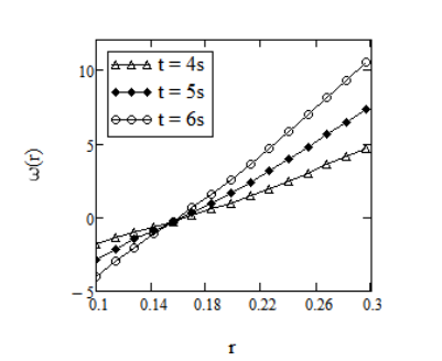
\(t\) and of the material parameters. Figure 1 shows the profile of the fluid motion at different values of time. From these figure one can clearly observe that velocity of the fluid increases with passing time. 
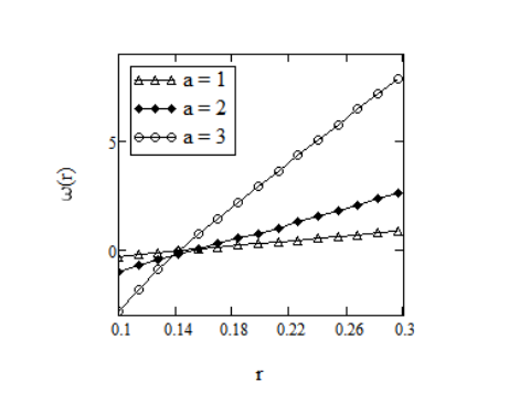
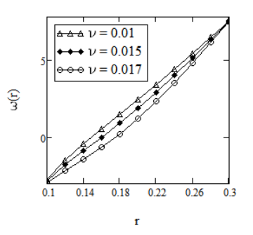
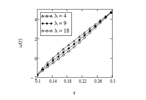
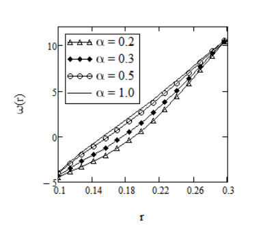
Effect of power parameter \(a\) on the velocity field is given in Figure 2. It shows that velocity of the fluid is an increasing function of \(a\). In Figures 3 and 4, it is shown that the laxation time \(\nu\) and \(\lambda\) has the same effect on the fluid motion. More exactly, velocity is an increasing function with respect to both \(\nu\) and \(\lambda\). Effect of fractional parameter \(\alpha\) on the fluid motion is represented in Figure 5, it is clearly seen that velocity of the fluid increases as fluid goes to Maxwell fluid.
Finally, for comparison, the diagrams of \(w(r,t)\) corresponding to fractional Maxwell, ordinary Maxwell and Newtonian fluids are together drawn in Figure 6 for the same values of the common material constants and time \(t\). The Newtonian fluid is the swiftest, while the fractional Maxwell fluid is the slowest. One thing is of worth mentioning that units of the material constants are SI units in all figures, and the roots \(r_{n}\) have been approximated by \(n\pi/(R_2-R_1)\).

Profiles of the velocity \(w(r,t)\) given by Eq. (23) for \(R_1=0.1,\,R_2=0.3,\,\Omega_1=-1,\,\Omega_2=1,\,a=2,\,\nu=0.003,\,\mu=2.916,\,\lambda=4,\,\alpha=0.5\) and different values of \(t\).

Profiles of the velocity \(w(r,t)\) given by Eq. (23)
for \(R_1=0.1,\,R_2=0.3,\,\Omega_1=-1,\,t=3,\,\Omega_2=1,\,\nu=0.003,\,\mu=2.916,\,\lambda=4,\,\alpha=0.5\) and different values of a.

Profiles of the velocity \(w(r,t)\) given by Eq. (23) for \(R_1=0.1,\,R_2=0.3,\,\Omega_1=-1,\,\Omega_2=1,\,t=5,\,a=2,\,\mu=2.916,\,\lambda=3,\,\alpha=0.4\) and different values of \(\nu\).

Profiles of the velocity \(w(r,t)\) given by Eq. (23)
for \(R_1=0.1,\,R_2=0.3,\,\Omega_1=-1,\,\Omega_2=1,\,a=2,\,t=4,\,\nu=0.03,\,\mu=2,916,\,\alpha=0.9\) and different values of \(\lambda\).

Profiles of the velocity \(w(r,t)\) given by Eq. (23)
for \(R_1=0.1,\,R_2=0.3,\,\Omega_1=-1,\,\Omega_2=1,\,a=2,\,t=6,\,\nu=0.003,\,\mu=2.916,\,\lambda=1.5\) and different values of \(\alpha\).

Profiles of the velocity \(w(r,t)\) corresponding to the Newtonian, Maxwell and fractional Maxwell fluids, for \(R_1=0.1,\,R_2=0.3,\,\Omega_1=-1,\,\Omega_2=1,\,a=2,\,t=6,\,\nu=0.0029,\,\mu=2.916,\,\lambda=1.8\) and \(\alpha=0.1.\)

Competing Interests

The author(s) do not have any competing interests in the manuscript.

References

  1. Rajagopal, K. R. (1993). Mechanics of non-Newtonian fluids. Pitman Research Notes in Mathematics Series, 129-129. [Google Scholor]
  2. Dunn, J. E., & Rajagopal, K. R. (1995). Fluids of differential type: critical review and thermodynamic analysis. International Journal of Engineering Science, 33(5), 689-729.[Google Scholor]
  3. Han, S. F. (2000) Constitutive equation and computational analytical theory Of non-Newtonian fluids, Science Press, Beijing. [Google Scholor]
  4. Podlubny, I. (1999). Fractional differential equations, Academic Press, San Diego. [Google Scholor]
  5. Friedrich, C. H. R. (1991). Relaxation and retardation functions of the Maxwell model with fractional derivatives. Rheologica Acta, 30(2), 151-158. [Google Scholor]
  6. Hilfer, R. (Ed.). (2000). Applications of fractional calculus in physics. World Scientific.[Google Scholor]
  7. Mingyu, X., & Wenchang, T. (2003). Representation of the constitutive equation of viscoelastic materials by the generalized fractional element networks and its generalized solutions. Science in China Series G: Physics Mechanics and Astronomy, 46(2), 145-157. [Google Scholor]
  8. Wenchang, T., & Mingyu, X. (2002). Plane surface suddenly set in motion in a viscoelastic fluid with fractional Maxwell model. Acta Mechanica Sinica, 18(4), 342-349. [Google Scholor]
  9. Wenchang, T., Wenxiao, P., & Mingyu, X. (2003). A note on unsteady flows of a viscoelastic fluid with the fractional Maxwell model between two parallel plates. International Journal of Non-Linear Mechanics, 38(5), 645-650. [Google Scholor]
  10. Hayat, T., Nadeem, S., & Asghar, S. (2004). Periodic unidirectional flows of a viscoelastic fluid with the fractional Maxwell model. Applied Mathematics and Computation, 151(1), 153-161. [Google Scholor]
  11. Qi, H., & Jin, H. (2006). Unsteady rotating flows of a viscoelastic fluid with the fractional Maxwell model between coaxial cylinders. Acta Mechanica Sinica, 22(4), 301-305. [Google Scholor]
  12. Qi, H., & Xu, M. (2007). Unsteady flow of viscoelastic fluid with fractional Maxwell model in a channel. Mechanics Research Communications, 34(2), 210-212. [Google Scholor]
  13. Fetecau, C., Fetecau, C., Jamil, M., & Mahmood, A. (2011). RETRACTED ARTICLE: Flow of fractional Maxwell fluid between coaxial cylinders. Archive of Applied Mechanics, 81(8), 1153-1163. [Google Scholor]
  14. Mahmood, A., Parveen, S., Ara, A., & Khan, N. A. (2009). Exact analytic solutions for the unsteady flow of a non-Newtonian fluid between two cylinders with fractional derivative model. Communications in Nonlinear Science and Numerical Simulation, 14(8), 3309-3319. [Google Scholor]
  15. Wood, W. P. (2001). Transient viscoelastic helical flows in pipes of circular and annular cross-section. Journal of non-newtonian fluid mechanics, 100(1), 115-126.[Google Scholor]
  16. Tong, D., Wang, R., & Yang, H. (2005). Exact solutions for the flow of non-Newtonian fluid with fractional derivative in an annular pipe. Science in China Series G: Physics Mechanics and Astronomy, 48(4), 485-495. [Google Scholor]
  17. Hayat, T., Khan, M., & Wang, Y. (2006). Non-Newtonian flow between concentric cylinders. Communications in Nonlinear Science and Numerical Simulation, 11(3), 297-305. [Google Scholor]
  18. Vieru, D., Akhtar, W., Fetecau, C., & Fetecau, C. (2007). Starting solutions for the oscillating motion of a Maxwell fluid in cylindrical domains. Meccanica, 42(6), 573-583. [Google Scholor]
  19. Akhtar, W., & Nazar, M. (2008). Exact solutions for the rotational flow of generalized Maxwell fluids in a circular cylinder. Bulletin mathématique de la Société des Sciences Mathématiques de Roumanie, 93-101. [Google Scholor]
  20. Wang, S.,& Xu, M. (2009). Axial Couette flow of two kinds of fractional viscoelastic fluids in an annulus. Nonlinear Analysis: Real World Applications, 10(2), 1087-1096.[Google Scholor]
  21. Khan, M., Ali, S. H., & Qi, H. (2009). Exact solutions of starting flows for a fractional Burgers’ fluid between coaxial cylinders. Nonlinear analysis: real world applications, 10(3), 1775-1783. [Google Scholor]
  22. Athar, M., Kamran, M., & Fetecau, C. (2010). Taylor-Couette flow of a generalized second grade fluid due to a constant couple. Nonlinear Analysis: Modelling and Control, 15(1), 3-13. [Google Scholor]
  23. Jamil, M.,& Fetecau, C. (2010). Helical flows of Maxwell fluid between coaxial cylinders with given shear stresses on the boundary. Nonlinear Analysis: Real World Applications, 11(5), 4302-4311.[Google Scholor]
  24. Zheng, L., Li, C., Zhang, X., & Gao, Y. (2011). Exact solutions for the unsteady rotating flows of a generalized Maxwell fluid with oscillating pressure gradient between coaxial cylinders. Computers & Mathematics with Applications, 62(3), 1105-1115. [Google Scholor]
  25. Imran, M., Kamran, M., & Athar, M. (2011). Exact analytical solutions for axial flow of a fractional second grade fluid between two coaxial cylinders. Theoretical and Applied Mechanics Letters, 1(2), 10-022002. [Google Scholor]
  26. Imran, M., Awan, A. U., Rana, M., Athar, M., & Kamran, M. (2012). Exact solutions for the axial Couette flow of a fractional Maxwell fluid in an annulus. ISRN Mathematical Physics, 2012, Article ID 209678, 15 pages.. [Google Scholor]
  27. L. Debnath and D. Bhatta, Integral Transforms and Their Applications (second ed.), Chapman and Hall/CRC Press, Boca Raton, 2007.[Google Scholor]
  28. Lorenzo, C. F., & Hartley, T. T. (1999). Generalized functions for the fractional calculus (Vol. 209424). National Aeronautics and Space Administration, Glenn Research Center.[Google Scholor]