Open Journal of Mathematical Sciences

Vol. 2 (2018), Issue 1, pp. 287 – 300
ISSN: 2523-0212 (Online) 2616-4906 (Print)
DOI: 10.30538/oms2018.0035

Analytical Technique for (2+1) Fractional Diffusion Equation with Nonlocal Boundary Conditions

Rahmatullah Ibrahim Nuruddeen\(^{1}\), Bashir Danladi Garba
Department of Mathematics, Federal University Dutse, Jigawa State, Nigeria. (N.I.N)
Department of Mathematics, Kano University of Science and Technology, Wudil, Kano-Nigeria.(B.D.G)

\(^{1}\)Corresponding Author: rahmatullah.n@fud.edu.ng

Received: April 5, 2018 – Accepted: September 12, 2018 – Published: October 7, 2018

Abstract

In the present article, a time fractional diffusion problem is formulated with special boundary conditions, specifically the nonlocal boundary conditions. This new problem is then solved by utilizing the Laplace transform method coupled to the well-known Adomian decomposition method after employing the modified version of Beilin’s lemma featuring fractional derivative in time. The Caputo fractional derivative is used. Some test problems are included.

Keywords:

fractional diffusion equation, nonlocal boundary conditions, decomposition method.

1. Introduction

Heat conduction problems frequently occur in many industrial processes thereby necessitating much attention from researchers. Of recent, these problems tend to be modelled with fractional order derivatives in either time or space variables or both. In light of this, the study of fractional differential equations [1, 2, 3] becomes vital in this regards. Moreover, many methods have been employed by many researchers to tackle varieties of heat conduction problems ranging from analytical down to approximate methods such that the novel series method for fractional diffusion equation by Yan et al. [4], an approximate decomposition method solution for a fractional diffusion-wave equation by Al-Khaled and Momani [5], the Adomian decomposition method for a fractional diffusion equation, nonlinear heat equation, heat equation with nonlocal boundary conditions and nonlinear diffusion equations, respectively [6, 7, 8, 9, 10]. Other methods include, the symmetry method for classifications of (2+1)-nonlinear heat equation by Ahmad et al. [11], the Sumudu Homotopy Perturbation Method (SHPM) for fractional KdV equations [12], the computational approach based on ADM [13], the Laplace transform method for fractional fluid flow and oscillatory process equations [14] and lastly the Wiener-Hopf method [15, 16, 17] for semi-infinite heat problems among others.

However, in the present article, a time fractional diffusion problem is formulated with special boundary conditions, specifically, the nonlocal boundary conditions. This new problem is aimed to be solved through utilizing the well-known Laplace transform method [18] alongside employing the Adomian decomposition method [7] in what is termed as the Laplace decomposition method, [19, 20, 21, 22, 23]. Further, in order to achieve this, a modification to Beilin's lemma [24] to feature fractional derivative in time variable will be given.

The paper is organized as follows: In Section 2, we present some basics about the fractional calculus. Section 3 gives the formulation of the problem under consideration. In Section 4, we give the analysis of the methodology and in Section 5, we present some application and results, and finally, Section 6 gives the conclusion.

Fractional Calculus and Some Definitions

In this section, we give some preliminary definitions of fractional calculus theory which will be used later on as follows:

Definition 2.1. [Caputo Fractional Derivative] The Caputo derivative of a casual function \(u(t)\) \((u(t)=0, \ t < 0)\) with \(\alpha>0\) is defined by [19]

\begin{equation} D^{\alpha}_t u(t)= \frac{1}{\Gamma(m-\alpha)} \int_{0}^{\infty} (t-s)^{m-\alpha-1}u^m(s) ds, \ (m-1 < \alpha\leqslant m). \end{equation}

(1)

Where \(\Gamma(.)\) is the well-known gamma function defined by \begin{equation*} (x-1)!=\Gamma(x)=\int_{0}^{\infty}e^{-t} t^{x-1} dt. \end{equation*} Some useful properties of the Caputo derivative are given below:

\(D^{\alpha}_t t^r=\frac{\Gamma(1+r)}{\Gamma(1+r-\alpha)} t^{r-\alpha},\)
\(D^{\alpha}_t \left[ c u(t)\right] = c D^{\alpha}_t u(t), \ \ c\) constant,
\(D^{\alpha}_t c = 0,\) \(c\) constant,
\(D^{\alpha}_t \left[ c u(t) + k v(t) \right] = c D^{\alpha}_t \left[ u(t) \right]+ k D^{\alpha}_t \left[ v(t) \right],\)
\(D^{\alpha}_t \left[ u(t) v(t) \right] = v(t) D^{\alpha}_t \left[ u(t) \right] + u(t) D^{\alpha}_t \left[ v(t) \right] .\)

For more, see [1, 2, 3].

Definition 2.2. [Laplace Transform for Caputo Fractional Derivative] The Laplace transform for Caputo fractional derivative is given by

\begin{equation} \mathcal{L}\{u^{\alpha}(t)\} =s^{\alpha}\mathcal{L}\{u(t)\}-\sum_{k=0}^{m-1}s^{\alpha-k-1}u^k(0), \ \ \ (m-1< \alpha\leqslant m). \end{equation}

(2)

Definition 2.3. [Mittag-Leffler Function] The one parameter Mittag-Leffler function is given by [2]

\begin{equation} E_\alpha(t)=\sum_{m=0}^{\infty} \frac{t^m}{\Gamma(\alpha m+1)}, \ \ \alpha>0, t \in \ \mathbb{C}. \end{equation}

(3)

Definition 2.4.[Formulation of the Problem] We consider the time-fractional 2-dimensional heat diffusion equation of the form

\begin{equation} \frac{\partial^\alpha u}{\partial t^\alpha}=\frac{\partial^2 u}{\partial x^2}+\frac{\partial^2 u}{\partial y^2}, \ \ \ \ \ 0< \alpha\leq 1, \end{equation}

(4)

subject to the initial condition

\begin{equation} u(x,y,0)=g(x,y), \ \ \ \ \quad x,y\in [0,l], \ 0< t\leq T, \end{equation}

(5)

and the nonlocal boundary conditions

\begin{equation} \int_{0}^{1}u(x,y,t)dx =0, \quad y=0 \\ \end{equation}

(6)

\begin{equation} \int_{0}^{1}u(x,y,t)dy =0, \quad x=0. \end{equation}

(7)

Furthermore, the function \(g(x,y)\) is assumed to satisfy the comparability conditions; that is \begin{equation*} \begin{split} g(0,0)& =0,\\ \int_{0}^{1}g(x,y)dx & =0, \quad y=0 \\ \int_{0}^{1}g(x,y)dy & =0, \quad x=0. \end{split} \end{equation*} Here, we give the following lemma by virtue of the modified Beilin's lemma [23] in Caputo fractional derivative sense to transform problem (4)-(7) to an equivalent boundary value problem with classical boundary conditions

Lemma 2.5. Problem (4)-(7) is equivalent to the following problem

\begin{equation} \left\{ \begin{array}{rcl} \frac{\partial^\alpha u}{\partial t^\alpha}=\frac{\partial^2 u}{\partial x^2}+\frac{\partial^2 u}{\partial y^2},\\ u(x,y,0) =g(x,y), \\ u(0,0,t) =0, \\ u_{xy}(l,0,t) +u_{xy}(0,l,t)\\-2u_{xy}(0,0,t)=0. \\ \end{array}\right. \end{equation}

(8)

Proof. Let \(u(x,t,t)\) be a solution of (4)-(7). Integrating (4) w.r.t `\(x\)' and `\(y\)' over \((0,l)\) respectively alongside utilizing (6)-(7), we get

\begin{equation} u_{x}(l,y,t) - u_{x}(0,y,t)=0, \ \ \ \ y=0, \end{equation}

(9)

and

\begin{equation} u_{y}(x,l,t) - u_{y}(y,0,t)=0, \ \ \ \ x=0. \end{equation}

(10)

Differentiating (9) w.r.t `\(y\)' at \(y=0\) and (10) w.r.t `\(x\)' at \(x=0\) and thereafter add them, we get

\begin{equation} u_{xy}(l,0,t) +u_{xy}(0,l,t)\\-2u_{xy}(0,0,t)=0. \end{equation}

(11)

Now let \(u(x,t,t)\) be a solution of problem (8), the we show the following

\begin{equation} \int_{0}^{1}u(x,y,t)dx =0, \ \ \ \ \forall t \in (0,T), \end{equation}

(12)

and

\begin{equation} \int_{0}^{1}u(x,y,t)dy =0, \ \ \ \ \forall t \in (0,T). \end{equation}

(13)

To show this, we integrate (4) w.r.t `\(x\)' and yields \begin{equation*} \frac{\partial}{\partial t}\int_{0}^{1}u(x,y,t)dx-\frac{\partial^2}{\partial x^2}\int_{0}^{1}u(x,y,t)dx-\frac{\partial^2}{\partial y^2}\int_{0}^{1}u(x,y,t)dx=0. \end{equation*} Thus, by virtue of the compatibility conditions, we get \begin{equation*} \int_{0}^{1}u(x,y,t)dx =0, \ \ \ \ \forall t \in (0,T).\\ \end{equation*} Similarly, \begin{equation*} \int_{0}^{1}u(x,y,t)dy =0, \ \ \ \ \forall t \in (0,T). \end{equation*}

3. Analysis of the Method

To illustrate the basic idea of the method, we consider a general nonlinear nonhomogeneous time-fractional partial differential equation with initial conditions of the following form:

\begin{equation} u^\alpha_t(x,t)= L\left(u(x,t)\right) +N\left(u(x,t)\right) + f(x,t), \ \ \ \alpha>0, \end{equation}

(14)

subject to the initial condition

\begin{equation} \begin{split} D^{k}_0 & u(x,0)=g_k (x), \ \ (k=0, 1,2,...n-1), \\ D^{n}_0 & u(x,0)=0, \ \ \ \ \ \ \ \ n=[\alpha],\\ \end{split} \end{equation}

(15)

where \(u^\alpha_t\) is the Caputo derivative of order \(\alpha\), and \(f(x,t)\) is the source function; \(L\) represents a linear fractional differential operator and \(N\) is the general nonlinear fractional differential operator.
The method first starts by taking the Laplace transform of equation (14) in \(t\), subject to the prescribed initial conditions given in equation (15), we obtain

\begin{equation} s^\alpha \mathcal{L}\{u(x,t)\}=\sum_{k=0}^{m-1}s^{\alpha-k-1}g_k(x)+ \mathcal{L}\left(L\left(u(x,t)\right) +N\left(u(x,t)\right) + f(x,t)\right), \end{equation}

(16)

\begin{equation} \mathcal{L}\{u(x,t)\}=\sum_{k=0}^{m-1}s^{-k-1}g_k(x)+ \frac{1}{s^\alpha} \mathcal{L}\left(L\left(u(x,t)\right) +N\left(u(x,t)\right) \right)+\frac{1}{s^\alpha}\left(\mathcal{L}(f(x,t))\right). \end{equation}

(17)

Now, taking the inverse Laplace transform of equation (17) and attaching the nonhomogeneous term with the initial conditions, yields

\begin{equation} \begin{split} u(x,t)=\sum_{k=0}^{m-1}\frac{t^k}{\Gamma(k+1)}g_k(x)+\mathcal{L}^{-1}\left(\frac{1}{s^\alpha}\left(\mathcal{L}(f(x,t)\right))\right)\\+\mathcal{L}^{-1}\left(\frac{1}{s^\alpha} \mathcal{L}\left(L\left(u(x,t)\right) +N\left(u(x,t)\right) \right)\right). \end{split} \end{equation}

(18)

Now, from equation (18), we assume the unknown function \(u(x,t)\) to have the series solution and the nonlinear term \(N\left(u(x,t)\right)\) by the Adomian polynomials [7];

\begin{equation} u(x,t)=\sum_{m=0}^{\infty}u_m(x,t), \ \ N\left(u(x,t)\right)= \sum_{m=0}^{\infty}A_m, \end{equation}

(19)

where \(A_m\)'s are the Adomian polynomials, see [7]. Thus, equation (18) becomes

\begin{equation} \begin{split} \sum_{m=0}^{\infty}u_m(x,t)=\sum_{k=0}^{m-1}\frac{t^k}{\Gamma(k+1)}g_k(x)+\mathcal{L}^{-1}\left(\frac{1}{s^\alpha}\left(\mathcal{L}(f(x,t)\right))\right)\\+\sum_{m=0}^{\infty}\mathcal{L}^{-1}\left(\frac{1}{s^\alpha} \mathcal{L}\left(L\left(u_m(x,t)\right) +A_m \right)\right) \end{split} \end{equation}

(20)

Thus we identify \(u_0 (x,t)\) with the initial condition term and the term resulting from the nonhomogeneous term; and the rest of the components \(u_m (x,t)\) are determined recursively as shown below:

\begin{equation} \left\{ \begin{array}{rcl} u_0(x,t)=\sum_{k=0}^{m-1}\frac{t^k}{\Gamma(k+1)}g_k(x)+\mathcal{L}^{-1}\left(\frac{1}{s^\alpha}\left(\mathcal{L}(f(x,t)\right))\right), & \quad m = 0. & \\ \\ u_{m+1}(x,t)=\mathcal{L}^{-1}\left(\frac{1}{s^\alpha} \mathcal{L}\left(L\left(u_m(x,t)\right) +A_m \right)\right), & \quad m \geq 0. \\ \end{array}\right. \end{equation}

(21)

4. Applications and Results

In this section, we apply the proposed method to two different time-fractional 2-dimensional heat diffusion equations and later illustrated the solutions graphically in figures 1a, 1b, 1c, 2a 2b and 2c with the aid of Mathematica software as follows:

Example 4.1. Consider the time-fractional 2-dimensional heat diffusion equation equation

\begin{equation} u_{t}^{\alpha}(x,t)= u_{xx}(x,t)+u_{yy}(x,t), \end{equation}

(22)

with the initial condition

\begin{equation} u(x,y,0)=\sin(x)\sin(y), \end{equation}

(23)

and the boundary conditions

\begin{equation} \begin{split} \int_{0}^{1}u(x,y,t)dx & =0, \quad y=0 \\ \int_{0}^{1}u(x,y,t)dy & =0, \quad x=0.\\ \end{split} \end{equation}

(24)

First, we transform our system (22)-(24) using Lemma 2.5 to obtain a system solvable by the Laplace decomposition method as follows:

\begin{equation} \frac{\partial^\alpha u}{\partial t^\alpha}=\frac{\partial^2 u}{\partial x^2}+\frac{\partial^2 u}{\partial y^2}, \end{equation}

(25)

subject to the new conditions \begin{equation*} \left\{ \begin{array}{rcl} u(x,y,0) =\sin(x)\sin(y), \\ u(0,0,t) =0, \\ u_{xy}(l,0,t) +u_{xy}(0,l,t)\\-2u_{xy}(0,0,t)=0. \\ \end{array}\right. \end{equation*} Then, on taking the Laplace transform of both sides of equation (25) subject to the initial condition, we obtain

\begin{equation} s^\alpha\mathcal{L}\{u(x,y,t)\}=s^{\alpha-1}\sin(x)\sin(y)+\mathcal{L}\{u_{xx}+u_{yy}\}, \end{equation}

(26)

\begin{equation} \mathcal{L}\{u(x,y,t)\}=\frac{1}{s}\sin(x)\sin(y)+\frac{1}{{s^\alpha}}\mathcal{L}\{u_{xx}+u_{yy}\}. \end{equation}

(27)

Taking the inverse Laplace transform of equation (27), we get

\begin{equation} u(x,y,t)=\sin(x)\sin(y)+\mathcal{L}^{-1} \{\frac{1}{{s^\alpha}}\mathcal{L}\{u_{xx}+u_{yy}\}. \end{equation}

(28)

Now, from equation (28), we assume the unknown function \(u(x,y,t)\) to have the series solution

\begin{equation} u(x,y,t)=\sum_{m=0}^{\infty}u_m(x,y,t), \end{equation}

(29)

Thus, equation (28) becomes

\begin{equation} \sum_{m=0}^{\infty}u_m(x,y,t)=\sin(x)\sin(y)+\mathcal{L}^{-1} \{\frac{1}{{s^\alpha}}\mathcal{L}\{\sum_{m=0}^{\infty}u_{m_{xx}}+u_{m_{yy}}\}\}. \end{equation}

(30)

Thus we identify \(u_0 (x,y,t)\) with the initial condition term that originate from the initial condition; and the rest of the components \(u_m (x,y,t)\) are determined recursively by:

\begin{equation} \left\{ \begin{array}{rcl} u_0(x,y,t)=\sin(x)\sin(y), & \quad m=0, \\ \\ u_{m+1}(x,y,t)=\mathcal{L}^{-1} \{\frac{1}{{s^\alpha}}\mathcal{L}\{u_{m_{xx}}+u_{m_{yy}}\}\}, & \quad m \geq 0. \end{array}\right. \end{equation}

(31)

We now obtain some few terms from equation (31) as follows

\begin{equation} u_0(x,y,t)=\sin(x)\sin(y), \end{equation}

(32)

\begin{equation} \begin{split} u_1(x,y,t)& =\mathcal{L}^{-1} \{\frac{1}{{s^\alpha}}\mathcal{L}\{u_{0_{xx}}+u_{0_{yy}}\}\}, \\ & =\mathcal{L}^{-1} \{\frac{1}{{s^\alpha}}\mathcal{L}\{-2\sin(x)\sin(y)\}\},, \\ & =\mathcal{L}^{-1} \{\frac{-2}{{s^{\alpha+1}}}\sin(x)\sin(y)\}, \\ & =\frac{-2t^\alpha}{\Gamma(\alpha+1)} \sin(x)\sin(y), \end{split} \end{equation}

(33)

\begin{equation} \begin{split} u_2(x,y,t)& =\mathcal{L}^{-1} \{\frac{1}{{s^\alpha}}\mathcal{L}\{u_{1_{xx}}+u_{1_{yy}}\}\}, \\ & =\mathcal{L}^{-1} \{\frac{1}{{s^\alpha}}\mathcal{L}\{\frac{4t^\alpha}{\Gamma(\alpha+1)} \sin(x)\sin(y)\}\}, \\ & =\mathcal{L}^{-1} \{\frac{4}{s^{2\alpha+1}} \sin(x)\sin(y)\}, \\ & =\frac{4t^{2\alpha}}{\Gamma(2\alpha+1)} \sin(x)\sin(y), \end{split} \end{equation}

(34)

\begin{equation} \begin{split} u_3(x,y,t)& =\mathcal{L}^{-1} \{\frac{1}{{s^\alpha}}\mathcal{L}\{u_{2_{xx}}+u_{2_{yy}}\}\}, \\ & =\mathcal{L}^{-1} \{\frac{1}{{s^\alpha}}\mathcal{L}\{\frac{-8t^{2\alpha}}{\Gamma(2\alpha+1)} \sin(x)\sin(y)\}\}, \\ & =\mathcal{L}^{-1} \{\frac{-8}{s^{3\alpha+1}} \sin(x)\sin(y)\}, \\ & =\frac{-8t^{3\alpha}}{\Gamma(3\alpha+1)} \sin(x)\sin(y), \end{split} \end{equation}

(35)

and so on. We therefore sum up the above iterations to get

\begin{eqnarray} \nonumber u(x,y,t) &=&\sum_{m=0}^{\infty}u_m(x,t)\\ \nonumber &=&\left(1-\frac{2t^{\alpha}}{\Gamma(\alpha+1)} + \frac{4t^{2\alpha}}{\Gamma(2\alpha+1)} -\frac{8t^{3\alpha}}{\Gamma(3\alpha+1)}+...\right)\sin(x)\sin(y),\\&& \end{eqnarray}

(36)

which leads to the exact solution

\begin{equation} u(x,y,t)=\sum_{m=0}^{\infty} \frac{(-2t)^m}{\Gamma(\alpha m+1)}\sin(x)\sin(y)= E_{\alpha} (-2t)\sin(x)\sin(y). \ \ \ \ \ \ \ \ \ \ \ \ \ \ \ \ \ \ \ \ \ \ \ \ \ \ \ \ \ \ \end{equation}

(37)

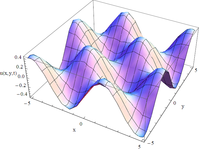
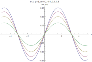
The graph of the solution of equation (37) is shown in Figure \(1a, 1b\) and \(1c\) as follows:

Figure 1a: Solution of equation (37) with at \(\alpha=0.5\) \(x,y \in (-5,5)\).

Figure 1b: Approxiamte Solution (only 3 terms) of equation(37) at \(\alpha=0.5\), \(x,y \in (-5,5)\).

Figure 1c: Solution of equation (37) at \(y=1, t=2\) with various \(\alpha’s\).

Example 4.2. Consider the time-fractional 2-dimensional heat diffusion equation equation

\begin{equation} u_{t}^{\alpha}(x,t)= u_{xx}(x,t)+u_{yy}(x,t), \end{equation}

(38)

with the initial condition

\begin{equation} u(x,y,0)=\sin(x+y), \end{equation}

(39)

and the boundary conditions

\begin{equation} \begin{split} \int_{0}^{1}u(x,y,t)dx & =0, \quad y=0 \\ \int_{0}^{1}u(x,y,t)dy & =0, \quad x=0.\\ \end{split} \end{equation}

(40)

Proceeding as above after obtaining the solvable system with the help of {\bf{Lemma 3.1}}, we get the solutions recursively as:

\begin{equation} \left\{ \begin{array}{rcl} u_0(x,y,t)=\sin(x+y), & \quad m=0 \\ \\ u_{m+1}(x,y,t)=\mathcal{L}^{-1} \{\frac{1}{{s^\alpha}}\mathcal{L}\{u_{m_{xx}}+u_{m_{yy}}\}\}, & \quad m \geq 0. \end{array}\right. \end{equation}

(41)

Some few terms from equation (41) are as follows

\begin{equation} u_0(x,y,t)=\sin(x+y), \end{equation}

(42)

\begin{equation} \begin{split} u_1(x,y,t)& =\mathcal{L}^{-1} \{\frac{1}{{s^\alpha}}\mathcal{L}\{u_{0_{xx}}+u_{0_{yy}}\}\}, \\ & =\mathcal{L}^{-1} \{\frac{1}{{s^\alpha}}\mathcal{L}\{-2\sin(x+y)\}\},, \\ & =\mathcal{L}^{-1} \{\frac{-2}{{s^{\alpha+1}}}\sin(x+y)\}, \\ & =\frac{-2t^\alpha}{\Gamma(\alpha+1)} \sin(x+y), \end{split} \end{equation}

(43)

\begin{equation} \begin{split} u_2(x,y,t)& =\mathcal{L}^{-1} \{\frac{1}{{s^\alpha}}\mathcal{L}\{u_{1_{xx}}+u_{1_{yy}}\}\}, \\ & =\mathcal{L}^{-1} \{\frac{1}{{s^\alpha}}\mathcal{L}\{\frac{4t^\alpha}{\Gamma(\alpha+1)} \sin(x+y)\}\}, \\ & =\mathcal{L}^{-1} \{\frac{4}{s^{2\alpha+1}} \sin(x+y)\}, \\ & =\frac{4t^{2\alpha}}{\Gamma(2\alpha+1)} \sin(x+y), \end{split} \end{equation}

(44)

\begin{equation} \begin{split} u_3(x,y,t)& =\mathcal{L}^{-1} \{\frac{1}{{s^\alpha}}\mathcal{L}\{u_{2_{xx}}+u_{2_{yy}}\}\}, \\ & =\mathcal{L}^{-1} \{\frac{1}{{s^\alpha}}\mathcal{L}\{\frac{-8t^{2\alpha}}{\Gamma(2\alpha+1)} \sin(x+y)\}\}, \\ & =\mathcal{L}^{-1} \{\frac{-8}{s^{3\alpha+1}} \sin(x+y)\}, \\ & =\frac{-8t^{3\alpha}}{\Gamma(3\alpha+1)} \sin(x+y), \end{split} \end{equation}

(45)

and so on. We therefore sum up the above iterations to get

\begin{equation} u(x,y,t) =\sum_{m=0}^{\infty}u_m(x,t)=\left(1-\frac{2t^{\alpha}}{\Gamma(\alpha+1)} + \frac{4t^{2\alpha}}{\Gamma(2\alpha+1)} -\frac{8t^{3\alpha}}{\Gamma(3\alpha+1)}+...\right)\sin(x+y), \end{equation}

(46)

which leads to the exact solution

\begin{equation} u(x,y,t)=\sum_{m=0}^{\infty} \frac{(-2t)^m}{\Gamma(\alpha m+1)}\sin(x+y)= E_{\alpha} (-2t)\sin(x+y). \ \ \ \ \ \ \ \ \ \ \ \ \ \ \ \ \ \ \ \ \ \ \ \ \ \ \ \ \ \ \end{equation}

(47)

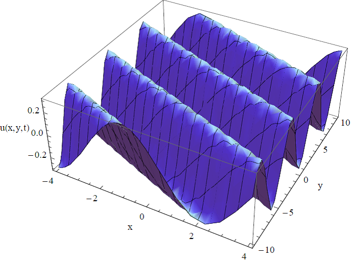
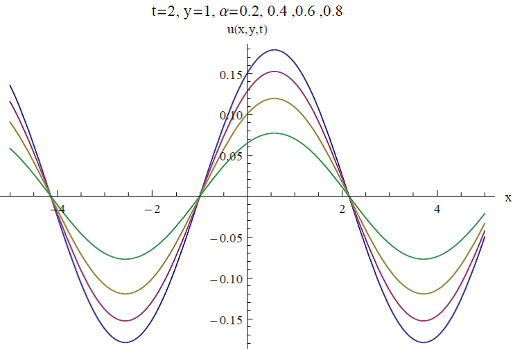
The graph of the solution of equation (47) is shown in Figure \(2a, 2b\) and \(2c\) as follows:

Figure 2a: Solution of equation (47) with at \(\alpha=0.5\) \(x,\in (-5,5), y \in (-3,3)\).

Figure 2b: Approxiamte Solution (only 3 terms) of equation(37) at \(\alpha=0.5\), \(x,\in (-5,5), y \in (-3,3)\).

5. Conclusion

In conclusion, a time fractional diffusion problem is formulated with nonlocal boundary conditions. This new problem is then solved through utilizing the Laplace transform method coupled to the well-known Adomian decomposition method after employing the modified version of Beilin's lemma featuring fractional derivative in time. Some test problems are solved and presented graphically with the aid of Mathematica software.

Competing Interests

The author(s) do not have any competing interests in the manuscript.

References

Debnath, L. (2003). Recent applications of fractional calculus to science and engineering. International Journal of Mathematics and Mathematical Sciences, 54, 3413-3442. [Google Scholor]
Kilbas, A. A., Srivastava, H. M. & Trujillo, J. J. (2006). Theory and Applications of Fractional Differential Equations. Elsevier, Amsterdam. [Google Scholor]
Abdon, A., & Dumitru, B. (2016). New fractional derivatives with nonlocal and non-singular kernel: Theory and application to heat transfer model. Thermal Science, 20(2), 763-769. [Google Scholor]
Yan, S. P., Zhong, W. P. & Yang, X. J. (2016). A novel series method for fractional diffusion equation within Caputo fractional derivative.Thermal Science, 20(3), S695-S699.[Google Scholor]
Al-Khaled, K. & Momani, S. (2005). An approximate solution for a fractional diffusion-wave equation using the decomposition method. Applied Mathematics and Computation, 2(15), 473-483. [Google Scholor]
Ray, S.S., & Bera, R.K. (2006). Analytical solution of a fractional diffusion equation by Adomian decomposition method. Applied Mathematics and Computation, 174, 329-336. [Google Scholor]
Adomian, G. (1988). A review of the decomposition method in applied mathematics. Journal of Mathematical Analysis and Applications, 135(2), 501-544. [Google Scholor]
Bokhari, A. H, Mohammad, G., Mustafa, M. T. & Zaman, F. D. (2009). Adomian decomposition method for a nonlinear heat equation with temperature dependent thermal properties. Mathematical Problems in Engineering. Volume 2009, Article ID 926086, 12 pages. [Google Scholor]
Bokhari, A. H, Mohammad, G., Mustafa, M. T. & Zaman, F. D. (2009). Solution of heat equation with nonlocal boundary conditions. International Journal of Mathematics and Computation, 3(J09), 100-113.[Google Scholor]
Wazwaz, A. M. (2001). Exact solutions to nonlinear diffusion equations obtained by the decomposition method. Applied Mathematics and Computation, 123(1),109-122. [Google Scholor]
Ahmad, A., Bokhari, A. H., Kara, A. H. & Zaman, F. D. (2008). Symmetry classifications and reductions of some classes of (2+1)-nonlinear heat equation. Journal of Mathematical Analysis and Applications, 339(1), 175-181. [Google Scholor]
Rehman, H., Saleem, M. S. & Ahmad, A. (2018). Combination of homotopy perturbation method (HPM) and double Sumudu transform to solve fractional KdV equations.Open Journal of Mathematical Sciences, 2(1), 29-38. [Google Scholor]
Bakodah, H. O. & Al-Zaid, N. A. (2018). Computational approaches to initial boundary value problems with Neumann boundary conditions. Journal of Taibah University for Science, 1-8.[Google Scholor]
Zakariya, Y. F., Afolabi, Y. O., Nuruddeen, R. I. & Sarumi, I. O. (2018). Analytical solutions to fractional fluid flow and oscillatory process models. Fractal and Fractional, 2(18), 1-12. [Google Scholor]
Nuruddeen, R. I., & Zaman, F. D. (2016). Heat conduction of a circular hollow cylinder amidst mixed boundary conditions. International Journal of Scientific Engineering and Technology, 5(1), 18-22. [Google Scholor]
Nuruddeen, R. I. & Zaman, F. D. (2016). Temperature distribution in a circular cylinder with general mixed boundary conditions. Journal of Multidisciplinary Engineering Science and Technology, 3 (1), 3653-3658. [Google Scholor]
Al-Duhaim, H. R., Nuruddeen, R. I. & Zaman, F. D. (2015). Thermal stress in a half-space with mixed boundary conditions due to time dependent heat source. IOSR Journal of Mathematics, 11(6), 19-25.[Google Scholor]
Laplace, P. S. (1820). Théorie Analytique des Probabilités, Lerch. Paris.
Caputo, M. (1999). Diffusion of fluids in porous media with memory. Geothermics 28, 113-130.[Google Scholor]
Eltayeb, H., Adem, K. & Said, M. (2015). Modified Laplace decomposition method for solving system of equations Emden-Fowler type. Journal of Computational and Theoretical Nanoscience, 12, 5297-5301.
Khuri, S. A. (2001). A Laplace decomposition algorithm applied to a class of nonlinear deferential equations. Journal of Applied Mathematics, 4(1), 141-155. [Google Scholor]
Islam, S., Khan, Y., Faraz, N. & Austin, F. (2010). Numerical solution of logistic differential equations by using the Laplace decomposition method. World Applied Sciences Journal, 8, 1100-1105. [Google Scholor]
Nuruddeen, R. I., Muhammad, L., Nass, A. M. & Sulaiman, T. A. (2018). A review of the integral transforms-based decomposition methods and their applications in solving nonlinear PDEs. Palestine Journal of Mathematics, 7, 262-280. [Google Scholor]
Beilin, S. A. (2001). Existence of solutions for one-dimensional wave equations with nonlocal boundary conditions. Electronic Journal of Differential Equations, 76, 1-8. [Google Scholor]