Effect of Magnetic Field on Double Convection Flow of Viscous Fluid over a Moving Vertical Plate with Constant Temperature and General Concentration by using New Trend of Fractional Derivative
1Abdus Salam School of Mathematical Sciences GC University Lahore, Pakistan.
2FAST, University Tun Hussein Onn Malaysia, 86400, Parit Raja, Batu Pahat, Johor State, Malaysia. And Public Authority of Applied Education and Training, College of Technological Studies, Applied Science Department, Shuwaikh, Kuwait.
3Department of Mathematics, COMSATS University Islamabad, Attock Campus, Pakistan.
4Department of Mathematical Sciences, Federal University of Technology, Akure, Nigeria.
This article presents, effects of fractional order derivative and magnetic field on double convection flow of viscous fluid over a moving vertical plate with constant temperature and general concentration. The model is fractionalized by using Caputo-Fabrizio derivative operator. Closed form solutions of the fluid velocity, concentration and temperature are obtained by means of the Laplace transform. Numerical computations and graphical illustrations are used in order to study the effects of the Caputo-Fabrizio time-fractional parameter , magnetic parameter , Prandtl and Grashof numbers on velocity field.
The enthusiasm in fluid mechanics is really meaningful in the presence of “transport phenomena, which is a significant feature in thermal, chemical, and mechanical engineering science. Several physical mechanism exists which can be used to transport thermal energy and chemical species through a phase and across boundaries of the phase. The three mechanisms for the heat transfer are diffusion, convection and radiation. Convection of heat transfer is further classified into three subsequent branches, namely; natural (free), forced, and mixed convection, depending upon the physical system initiating the motion of the fluid.
Free convection flows resulting from the heat and mass transfer driven by the combined buoyancy effect due to temperature and concentration variations have been extensively studied, due to their various applications in geosciences, chemical engineering, and industrial activities as food processing and polymer production. Other multiple areas of applications such as: heat transfer from transmission lines and pipes, heat conduction from electrical devices, heat debauchery from the spiral refrigerator element to surrounding air, heat transfer from a heater, heat transfer in nuclear energy poles, extrusion and wiredrawing, atmospheric and oceanic circulation, etc., have been studied by Jaluria [1]. Free convection problems are usually formulated under different situations like constant surface temperature, ramped temperature at the wall or surface heat flux [2].
Generally, the mass transfer due to the concentration differences affects the rate of heat transfer. The driving force for the free convection is buoyancy so its effects cannot be neglected when the fluid velocity is small and temperature difference between the surface and ambient fluid is large enough [3, 4, 5].
Electrically conducting fluids also have received much attention from the researchers due to their large scale applications in industrial appliances. The magneto hydrodynamics (MHD) has its own practical applications, such as the cooling of nuclear reactors by liquid sodium and induction flow meter, which depends on the potential difference in the fluid in the direction perpendicular to the motion and to the magnetic field [6].
The influence of magnetic field on the free convection flow is significant in liquid metals, electrolytes and ionized gases. The work of Soundalgekar et al. [7] is seemed to be the first on mass transfer and magnetic effects. The study of MHD in the free convection has attracted the interest of many researchers in view of its applications in geophysics and astrophysics [8].
The role of “Fractional Calculus” which is now a day’s called calculus of 21th century in modern sciences and engineering is very significant. The tools devised in the subject is used in past few decades to provide solutions to hundreds of real world problems. Researchers are interested to solve scientific problems using the techniques developed in fractional calculus. In the recent times, fractional calculus has been extended to several directions for instance fractional-order multipoles in the electromagnetism, electrochemistry, models in mathematical biology, finance, fluid flows tracers, signal processing in engineering, applied mathematics, bio-engineering and fluid dynamics [9]. Many researchers in fluid dynamics widely used fractional derivative models to study the viscoelastic materials such as polymers in glass transition. It is vital to bring in light the fact that fractional derivative generalizations of one dimensional viscoelastic models have seen to be more useful in modeling the response linear regime [10]. This generalization is in good agreement with the second law of thermodynamics.
The fractional derivative operators used up till now, are Riemann-Liouville fractional derivative and Caputo fractional derivative operator [11]. It is observed by many researchers that application of these operators exhibit difficulties, such as Riemann-Liouville fractional derivative of constant functions is not zero, and its Laplace transform contain terms without physical significance. Caputo fractional derivative has eliminated these difficulties, but the kernel in its definition is a singular function. The results that are been found using these operators are expressed in complicated forms involving some generalized functions.
Recently, Caputo and Fabrizio gave a new expression for fractional derivative operator with an exponential kernel without singularities. The Caputo-Fabrizio temporal-fractional derivative is suitable in the use of the Laplace transform. Shah et al. [12]applied the idea of the Caputo-Fabrizio fractional derivatives to generalize the starting flow of second grade fluid over a vertical plate and obtained the exact solutions using the Laplace transform technique. Some other recent studies can be found in [13, 14, 15, 16, 17] and the references therein.
2. Mathematical formulation of the problem
The unsteady magneto-hydrodynamic flow of viscous incompressible fluid past an infinite vertical plate and constant temperature and variable mass diffusion has been studied. Initially, the plate and the fluid are at the same temperature \(T_{\infty}\) in the stationary condition with concentration level \(C_{\infty}\) at all the points. At time \(t=0^{+}\), the plate is moving with a velocity \(U_{0}f(t)\) in its own plane and the temperature of the plate is constant \(T_{w}\) as well species concentration is raised or lowered to the value \(C_{\infty}+C_{w}g(t)\) with time. \(U_{0}\) is a constants with dimension of velocity while the dimensionless functions \(f(\cdot)\) and \(g(\cdot)\) are piecewise continuous of exponential order at infinity and \(f(0)=g(0)=0\) .
We made the following assumptions:
All fluid physical properties are considered to be constant except the influence of the body force terms.
Applied magnetic field of uniform strength \(B_{0}\) is normal to the plate.
The fluids conducting property is supposed to be slight and hence the magnetic Reynolds number is lesser than unity, the induced magnetic field is small in comparison with the transverse magnetic field.
It is further supposed that there is no applied voltage, as the electric field is absent.
Viscous dissipation and Joule heating in energy equation are neglected.
According to Boussinesq’s approximation, the unsteady flow is governed by the following set of equations:
Here, we have to developed fractional model, replacing the time derivative in Eqs. (8), (9) and (10), with time-fractional derivatives, we obtain the following fractional differential equations
where \(\gamma=\frac{1}{1-\alpha}\), \(\overline{T}(y,q)\) , is the Laplace transform of \(T(y,t)\) and \(q\) is the transform variable.
The solution of the partial differential equation (18) by using conditions in equation (19), we obtain
where \(\frac{1}{1-\alpha}\),\(\overline{C}(y,q)\) and \(G(q)\) are the Laplace transform of \(C(y,t)\) respectively \(g(t)\) and \(q\) is the transform variable.
The solution of the partial differential equation (22) by using conditions in equation (23), we obtain
where \(g'(t)=L^{-1}\{qG(q)\}\) , \(“ \ast “\) represent the convolution product and \(F_{1}(y,q,a,b,c),\) \(f_{1}(y,t,a,b,c)\) are defined in Appendix.
3.3. Calculation for velocity
Taking Laplace transform of Eqs. (14), \((12)_1\), \((13)_1\), using initial condition Eq. \((11)_1\), by introducing Eqs. (20) and (24), we obtain
where \(F(q)\) is the Laplace transform of \(f(t)\) .
The solution of the partial differential equation (27) subject to conditions in equation (28) can be written in the following suitable form as
where \(\displaystyle a_{1}=M-S\), \(\displaystyle a_{2}=a_{3}[(1-Pr)\gamma+a_{1}]\), \(\displaystyle a_{3}=\frac{1}{\alpha\gamma}\), \(\displaystyle a_{4}=\frac{a_{2}}{a_{1}}\), \(a_{5}=\frac{a_{1}-a_{2}a_{3}}{a_{1}a_{3}}\), \(b_{1}=M-\lambda\),
\(\displaystyle a_{2}=a_{3}[(1-Sc)\gamma+b_{1}]\), \(\displaystyle b_{3}=\frac{b_{1}}{b_{2}}\), \(\displaystyle b_{4}=\frac{b_{2}-a_{3}b_{1}}{a_{3}b_{2}}\)
and \(F_{1}(y,q,a,b,c)\) is defined in the Appendix.
Taking inverse Laplace transform of Eqs. (29), (30) and (31), we obtain
and \(f_{1}(y,t,a,b,c),\) is defined in Appendix and “\(\ast\)” represent the convolution product.
4. Numerical results and discussions
In order to obtain some information on the fluid flow parameters, we have made several numerical simulations using Mathcad software. Obtained results are presented in the graphs from Figures.1- 6. All the parameters and profiles are dimensionless.
We were interested, to analyze the influence of the fractional parameter \(\alpha\) with different values of time \(t\) , magnetic parameter \(M\) , Prandtl number \(Pr\) and Grashof number \(Gr\) on velocity field in order to study the flow behavior.
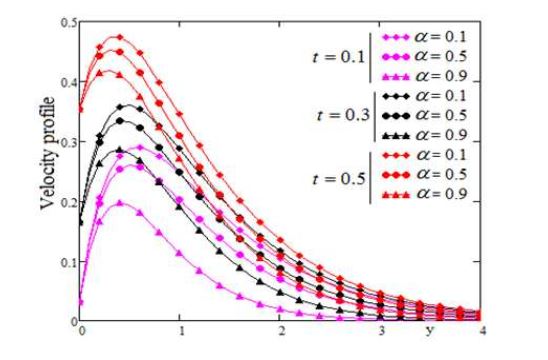
In Figure 1, we present the influence of the fractional parameter \(\alpha\) with small time \(t\) on velocity profile. It is observe that by increasing the value of the fractional parameter the velocity is decreases with small values of time and by increasing the time the velocity increase.
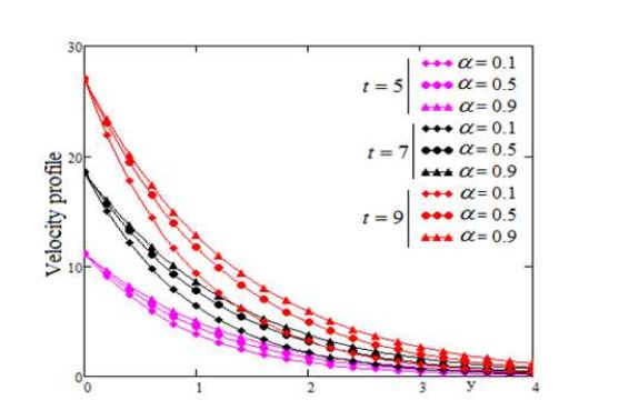
In Figure 2, we present the influence of the fractional parameter \(\alpha\) with large time \(t\) on velocity profile. It is observe that by increasing the value of the fractional parameter the velocity is increases with large values of time and by increasing the time the velocity increase.
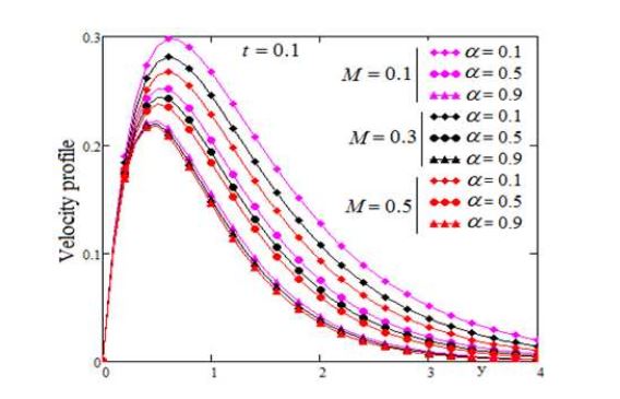
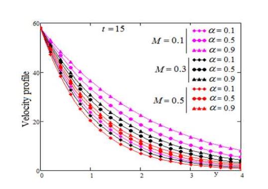
The effect of magnetic field for small and large values of time on velocity profile is presented in Figure 3, respectively Figure 4. It is observe that by increasing the magnetic field the velocity is decreases as which is expected for small as well as for large time.
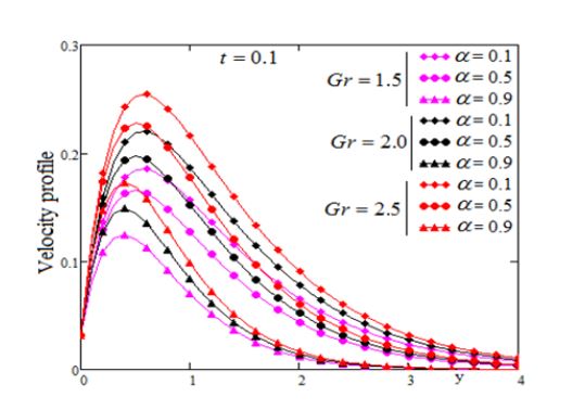
The effect of Prandtl number \(Pr\) and Grashof number \(Gr\) are presented in Figs. 5 and 6, respectively. It is observe that the velocity decrease by increasing the Prandtl”number \(Pr\) and increase by increasing the values of \(Gr\).
Figure 1. Profile of dimensionless velocity versus \(y\) for \(\alpha\) variation with \(Pr=0.7, S=5, Sc=0.8, \lambda=4, Gr=3, Gm=0.9, M=0.4\) and different small values of time \(t\).Figure 2. Profile of dimensionless velocity versus \(y\) for \(\alpha\) variation with \(Pr=0.7, S=5, Sc=0.8, \lambda=4, Gr=3, Gm=0.9, M=0.4\) and different large values of time \(t\).Figure 3. Profile of dimensionless velocity versus \(y\) for \(\alpha\) variation with \(Pr=0.7, S=5, Sc=0.8, \lambda=4, Gr=3, Gm=0.9,\) and different values of \(M\) for small time.Figure 4. Profile of dimensionless velocity versus \(y\) for \(\alpha\) variation with \(Pr=0.7, S=5, Sc=0.8, \lambda=4, Gr=3, Gm=0.9,\) and different values of \(M\) for large time.Figure 5. Profile of dimensionless velocity versus \(y\) for \(\alpha\) variation with \(M=0.4, S=5, Sc=0.8, \lambda=4, Gr=3, Gm=0.9,\) and different values of \(Pr\).Figure 6. Profile of dimensionless velocity versus \(y\) for \(\alpha\) variation with \(Pr=0.7, S=5, Sc=0.8, \lambda=4, Gm=0.9, M=0.4\) and different values of \(Gr\).
5. Conclusions
This aim of this article presents, the effects of fractional order derivative and magnetic field on double convection flow of viscous fluid over a moving vertical plate with constant temperature and general concentration. Numerical computations and graphical illustrations are used in order to study the effects of the Caputo-Fabrizio time-fractional parameter \(\alpha\), magnetic parameter \(M\), Prandtl and Grashof number on velocity field. The follow important points are observed
By increasing the value of the fractional parameter the velocity is decreases with small values of time and by increasing the time the velocity increase.
By increasing the value of the fractional parameter the velocity is increases with large values of time and by increasing the time the velocity increase.
By increasing the magnetic field the velocity is decreases.
The velocity decrease by increasing the Prandtl number \(Pr\).
The velocity increase by increasing the values of \(Gr\).
The author(s) do not have any competing interests in the manuscript.
References
Jaluria, Y. (1980). Natural convection: heat and mass transfer (Vol. 5). Pergamon. [Google Scholor]
Kays, W. M., Crawford, M. E., & Weigand, B. (2005). Convective Heat and Mass Transfer. McGraw-Hill Series in Mechanical Engineering. McGraw Hill. [Google Scholor]
Ghoshdastidar, P. S. (2004). Heat Transfer. Oxford University Press, UK.
Imran, M. A., Khan, I., Ahmad, M., Shah, N. A., & Nazar, M. (2017). Heat and mass transport of differential type fluid with non-integer order time-fractional Caputo derivatives. Journal of Molecular Liquids, 229, 67-75. [Google Scholor]
Fetecau, C., Vieru, D., Fetecau, C., & Pop, I. (2015). Slip effects on the unsteady radiative MHD free convection flow over a moving plate with mass diffusion and heat source. The European Physical Journal Plus, 130(1), 6. [Google Scholor]
Sharma, B. R., & Nath, K. (2013). Effects of Magnetic Field and Variation of Viscosity and Thermal Conductivity on Separation of a Binary Fluid Mixture over a Continuously Moving Surface. International Journal of Innovative Research in Science, Engineering and Technology, 2(11), 6516-6524. [Google Scholor]
Soundalgekar, V. M., Gupta, S. K., & Birajdar, N. S. (1979). Effects of mass transfer and free convection currents on MHD Stokes’ problem for a vertical plate. Nuclear Engineering and Design, 53(3), 339-346.[Google Scholor]
Kumar, A. V., Goud, Y. R., Varma, S. V. K., & Raghunath, K. (2012). Thermal diffusion and radiation effects on unsteady MHD flow through porous medium with variable temperature and mass diffusion in the presence of heat source/sink. Advances in Applied Science Research, 3(3), 1494-1506. [Google Scholor]
Ahmed, N., Vieru, D., Fetecau, C., & Shah, N. A. (2018). Convective flows of generalized time-nonlocal nanofluids through a vertical rectangular channel. Physics of Fluids, 30(5), 052002.[Google Scholor]
Shakeel, A., Ahmad, S., Khan, H., & Vieru, D. (2016). Solutions with Wright functions for time fractional convection flow near a heated vertical plate. Advances in Difference Equations, 2016(1), 51. [Google Scholor]
Zafar, A. A., & Fetecau, C. (2016). Flow over an infinite plate of a viscous fluid with non-integer order derivative without singular kernel. Alexandria Engineering Journal, 55(3), 2789-2796 [Google Scholor]
Shah, N. A., & Khan, I. (2016). Heat transfer analysis in a second grade fluid over and oscillating vertical plate using fractional Caputo–Fabrizio derivatives. The European Physical Journal C, 76(7), 362. [Google Scholor]
Khan, I., Shah, N. A., Mahsud, Y., & Vieru, D. (2017). Heat transfer analysis in a Maxwell fluid over an oscillating vertical plate using fractional Caputo-Fabrizio derivatives. The European Physical Journal Plus, 132(4), 194. [Google Scholor]
Shah, N., Ahmed, N., Elnaqeeb, T., & Rashidi, M. M. (2018). Magnetohydrodynamic Free Convection Flows with Thermal Memory over a Moving Vertical Plate in Porous Medium. Journal of Applied and Computational Mechanics.[Google Scholor]
Atangana, A., & Koca, I. (2016). On the new fractional derivative and application to nonlinear Baggs and Freedman model. J. Nonlinear Sci. Appl, 9(0), 5. [Google Scholor]
Alkahtani, B. S. T., & Atangana, A. (2016). Controlling the wave movement on the surface of shallow water with the Caputo–Fabrizio derivative with fractional order. Chaos, Solitons & Fractals, 89, 539-546. [Google Scholor]
Caputo, M., & Fabrizio, M. (2015). A new definition of fractional derivative without singular kernel. Progr. Fract. Differ. Appl, 1(2), 1-13. [Google Scholor]