Fixed point results for the complex fractal generation in the S-iteration orbit with s-convexity

1. Introduction

Mandelbrot and Julia sets are some of the best known illustrations of a highly complicated chaotic systems generated by a very simple mathematical process. They were introduced by Benoit Mandelbrot in the late 1970's [1], but Julia sets were studied much earlier, namely in the early 20th century by French mathematicians Pierre Fatou and Gaston Julia. Mandelbrot working at IBM has studied their works and plotted the Julia sets for \(z^2 + c\) and corresponding to them the Mandelbrot set. He was surprised by the result that he obtained. Since then many mathematicians have studied different properties of Mandelbrot and Julia sets and proposed various generalizations of those sets. The first and the most obvious generalization was the use of \(z^p + c\) function instead of the quadratic one used by Mandelbrot [2, 3]. Then some other types of functions were studied: rational [4], transcendental [5], elliptic [6], anti-polynomials [7] etc. Another step in the studies on Mandelbrot and Julia sets was the extension from complex numbers to other algebras, e.g., quaternions [8], octonions [9], bicomplex numbers [10] etc.
Another interesting generalization of Mandelbrot and Julia sets is the use of the results from fixed point theory. In the fixed point theory there exist many approximate methods of finding fixed points of a given mapping, that are based on the use of different feedback iteration processes. These methods can be used in the generalization of Mandelbrot and Julia sets. In 2004, Rani and Kumar [11, 12] introduced superior Julia and Mandelbrot sets using Mann iteration scheme. Chauhan et al. in [13] introduced the relative superior Julia sets using Ishikawa iteration scheme. Also, relative superior Julia sets, Mandelbrot sets and tricorn, multicorns by using the \(S\)-iteration scheme were presented in [14, 15]. Recently, Ashish et al. in [16] introduced Julia and Mandelbrot sets using the Noor iteration scheme, which is a three-step iterative procedure. The junction of a \(s\)-convex combination [17] and various iteration schemes was studied in many papers. Mishra et al. [18, 19] developed fixed point results in relative superior Julia sets, tricorn and multicorns by using the Ishikawa iteration with \(s\)-convexity. In [20] Kang et al. introduced new fixed point results for fractal generation using the implicit Jungck-Noor orbit with \(s\)-convexity, whereas Nazeer et al. in [21]NKTS15} used the Jungck-Mann and Jungck-Ishikawa iterations with \(s\)-convexity. The use of Noor iteration and \(s\)-convexity was shown in [22].
In this paper, we present some fixed point results for Julia and Mandelbrot sets by using the \(S\)-iteration scheme with \(s\)-convexity. We derive the escape criteria for quadratic, cubic and the \((k+1)\)th degree complex polynomial.
The remainder of this paper is outlined as follows. In Sec. 2 we present some basic definitions used in the paper. Next, in Sec.3, we present the main results of this paper, namely we prove the escape criteria for the quadratic, cubic and the \((k+1)\)th degree complex polynomial in the \(S\)-iteration with \(s\)-convexity. Some graphical examples of complex fractals generated using the escape criteria are presented in Sec.4. The paper ends with some concluding remarks and future work (Sec.5).

2. Preliminaries

Definition2.1. (see [23], Julia set) Let \(f: \mathbb{C} \rightarrow \mathbb{C}\) be a polynomial of degree \(\geq 2\). Let \(F_{f}\) be the set of points in \(\mathbb{C}\) whose orbits do not converge to the point at infinity, i.e., \(F_{f} = \{z \in \mathbb{C}: \{\left\vert f^{n}(z)\right\vert \}_{n=0}^{\infty} \text{ is bounded} \}.\) \(F_{f}\)\ is called as filled Julia set of the polynomial \(f\). The boundary points of \(F_{f}\) are called the points of Julia set of the polynomial \(f\) or simply the Julia set.

Definition 2.2.(see [24], Mandelbrot set) The Mandelbrot set \(M\) consists of all parameters \(c\) for which the filled Julia set of \(Q_{c}(z)=z^{2}+c\) is connected, i.e.,

In fact, \(M\) contains an enormous amount of information about the structure of Julia sets. The Mandelbrot set \(M\) for the quadratic \(Q_{c}(z)=z^{2}+c\) can be equivalently defined in the following way: We choose the initial point \(0\), because \)0\) is the only critical point of \(Q_{c}\), i.e., \(Q_{c}'(0) = 0\).

Definition 2.3. Let \(C \subset \mathbb{C}\) be a non-empty set and \(f:C\rightarrow C\). For any point \(z_{0} \in C\) the Picard orbit is defined as the set of iterates of the point \(z_{0}\), i.e.,

where the orbit \(O(f, z_{0})\) of \(f\) at the initial point \(z_{0}\) is the sequence \(\{f^{n}(z_{0})\}_{n = 1}^{\infty}\).

Definition 2.4.(see [25], \(S\)-iteration orbit) Consider a sequence \(\{z_{n}\}\) of iterates for initial point \(z_{0}\in C\) such that

where \(n = 0, 1, 2, \ldots\) and \(\gamma_{n}, \delta_{n} \in (0, 1]\). This sequence of iterates is called the \(S\) orbit, which is a function of four arguments \((f, z_{0}, \gamma_{n}, \delta_{n})\) and we will denote it by \(SO(f, z_{0}, \gamma_{n}, \delta_{n})\).

In [14] Kang et al. have proved the escape criterion for the Mandelbrot and Julia sets in \(S\)-orbit.

Theorem 2.5.[Escape Criterion for \(S\)-iteration] Let \(Q_c(z) = z^{k+1} + c\), where \(k = 1, 2, 3, \ldots\) and \(c \in \mathbb{C}\). Iterate \(Q_c\) using \eqref{eq:s} with \(\gamma_n = \gamma, \delta_n = \delta\), where \(\gamma, \delta \in (0, 1]\). Suppose that

then there exist \(\lambda > 0\) such that \(\left\vert z_{n}\right\vert >(1+\lambda )^{n}\left\vert z\right\vert \) and \(\left\vert z_{n}\right\vert \rightarrow \infty \) as \(n \rightarrow \infty\).

3. Main results

In each of the two steps of \(S\)-iteration we use a convex combination of two elements. In the literature we can find some generalizations of the convex combination. One of such generalizations is the \(s\)-convex combination.

Definition 3.1.[\(s\)-convex combination [17]] Let \(z_1, z_2, \ldots, z_n \in \mathbb{C}\) and \(s \in (0, 1]\). The \(s\)-convex combination is defined in the following way:

where \(\lambda_k \geq 0\) for \(k \in \{ 1, 2, \ldots, n \}\) and \(\sum_{k = 1}^{n} \lambda_k = 1\).

Let us notice that the \(s\)-convex combination for \(s = 1\) reduces to the standard convex combination. Now, we will replace the convex combination in the \(S\)-iteration with the \(s\)-convex one. Let \(Q_c\) be a polynomial and \(z_0 \in \mathbb{C}\). We define the \(S\)-iteration with \(s\)-convexity as follows: where \(n = 0, 1, 2, \ldots\) and \(\gamma, \delta, s \in (0, 1]\). We will denote the \(S\)-iteration with \(s\)-convexity by \(SO_s(f, z_0, \gamma, \delta, s)\). In the following subsections we prove escape criteria for some classes of polynomials using the \(S\)-iteration with \(s\)-convexity.

3.1. Escape criterion for quadratic function

Theorem 3.2. Assume that \(|z|\geq |c|>\frac{2}{s\gamma }\) and \(|z|\geq |c|>\frac{2}{s\delta }\), where \(\gamma, \delta, s \in (0, 1]\) and \(c \in \mathbb{C}\). Let \(z_0 = z\). Then for (7) with \(Q_c(z) = z^2 + c\) we have \(|z_{n}| \rightarrow \infty\) as \(n \rightarrow \infty\).

Proof. Consider \[ \left\vert w\right\vert =\left\vert (1-\delta )^{s}z+\delta^{s}Q_{c}(z)\right\vert. \] For \(Q_{c}(z)=z^{2}+c\), \begin{eqnarray*} \left\vert w\right\vert &=&\left\vert (1-\delta )^{s}z+\delta^{s}(z^{2}+c)\right\vert \\ &=&\left\vert (1-\delta )^{s}z+(1-(1-\delta ))^{s}(z^{2}+c)\right\vert. \end{eqnarray*} By binomial expansion upto linear terms of \(\delta \) and \((1-\delta ),\) we obtain

In the second step of the \(S\)-iteration with \(s\)-convexity we have By binomial expansion upto linear terms of \(\gamma \) and \((1-\gamma ),\) we obtain Since \(|z| > 2/(s \delta)\), which implies \(s\delta |z| > 2\) and \((s\delta |z|-1)^{2} >1\). Thus Using (11) in (10) we have \begin{eqnarray*} \left\vert z_{1}\right\vert &\geq &\left\vert (1-s\gamma )(z^{2}+c)+s\gamma(\delta |z|^{2}+c)\right\vert \\ &=&\left\vert s\gamma \delta \left\vert z\right\vert ^{2}+(1-s\gamma)z^{2}+(1-s\gamma )c+s\gamma c\right\vert \\ &=&\left\vert s\gamma \delta \left\vert z\right\vert ^{2}+(1-s\gamma)z^{2}+c\right\vert \\ &\geq & s \gamma \delta \left\vert z\right\vert ^{2}-\left\vert (s\gamma-1)z^{2}\right\vert -\left\vert c\right\vert \text{ } \\ &\geq &s\gamma \delta \left\vert z\right\vert ^{2}-(s\gamma -1)\left\vert z^{2}\right\vert -\left\vert z\right\vert \text{ }(\because \left\vert z\right\vert >\left\vert c\right\vert ) \\ &= &\left\vert z\right\vert \left( (s\gamma \delta -s\gamma +1)\left\vert z\right\vert -1\right). \end{eqnarray*} Because \(|z| > 2/(s\gamma)\) and \(|z| > 2/(s\delta)\), so \[ |z|>\frac{2}{s\gamma \delta }>\frac{2}{s\gamma \delta -s\gamma +1}, \] which implies \[ (s\gamma \delta -s\gamma +1)|z|-1>1. \] Therefore, there exists \(\lambda > 0\), such that \((s \gamma \delta -\gamma +1)|z|-1>1+\lambda >1.\) Consequently \begin{equation*} |z_{1}| > (1+\lambda ) |z|. \end{equation*} We may apply the same argument repeatedly to obtain: \begin{eqnarray*} \left\vert z_{2}\right\vert &>&(1+\lambda )^{2}\left\vert z\right\vert, \\ &&\vdots \\ \left\vert z_{n}\right\vert &>&(1+\lambda )^{n}\left\vert z\right\vert. \end{eqnarray*} Hence, \(\left\vert z_{n}\right\vert \rightarrow \infty \) as \(n\rightarrow \infty\). This completes the proof.

Corollary 3.3. Suppose that

then the orbit \(SO_s(Q_{c}, 0, \gamma, \delta, s)\) escapes to infinity.

The following corollary is the refinement of the escape criterion.

Corollary 3.4.[Escape Criterion] Let \(\gamma, \delta, s \in (0, 1]\). Suppose that

then there exist \(\lambda > 0\) such that \(\ \left\vert z_{n}\right\vert >(1+\lambda)^{n}\left\vert z\right\vert \) and \(\left\vert z_{n}\right\vert \rightarrow \infty \) as \(n\rightarrow \infty .\)

3.2. Escape criterion for cubic function

Theorem 3.5. Assume that \(|z| \geq |c|> (\frac{2}{s\gamma })^{\frac{1}{2}}\) and \(|z|\geq |c| > (\frac{2}{s\delta })^{\frac{1}{2}}\), where \(c \in \mathbb{C}\) and \(\gamma, \delta, s \in (0, 1]\). Let \(z_0 = z\). Then for (7) with \(Q_c(z) = z^3 + c\) we have \(\left\vert z_{n}\right\vert \rightarrow \infty\) as \(n \rightarrow \infty\).

Proof. Consider \[ \left\vert w\right\vert =\left\vert (1-\delta )^{s}z+\delta^{s}Q_{c}(z)\right\vert. \] For \(Q_{c}(z)=z^{3}+c\), we have \begin{eqnarray*} \left\vert w\right\vert &=&\left\vert (1-\delta )^{s}z+\delta^{s}(z^{3}+c)\right\vert \\ &=&\left\vert (1-\delta )^{s}z+(1-(1-\delta ))^{s}(z^{3}+c)\right\vert. \end{eqnarray*} By binomial expansion upto linear terms of \(\delta \) and \((1-\delta ),\) we obtain

In the second step of the \(S\)-iteration with \(s\)-convexity we have By binomial expansion upto linear terms of \(\gamma \) and \((1-\gamma ),\) we obtain Since \(|z| > (2/(s \delta))^{\frac{1}{2}}\), which implies \(s\delta |z|^{2}>2\) and \((s\delta |z|^{2}-1)^{3} >1\). Thus Using (17) in (16) we have \begin{eqnarray*} \left\vert z_{1}\right\vert &\geq &\left\vert (1-s\gamma )(z^{3}+c)+s\gamma(\delta |z|^{3}+c)\right\vert \\ &=&\left\vert s\gamma \delta \left\vert z\right\vert ^{3}+(1-s\gamma)z^{3}+(1-s\gamma )c+s\gamma c\right\vert \\ &=&\left\vert s\gamma \delta \left\vert z\right\vert ^{3}+(1-s\gamma)z^{3}+c\right\vert \\ &\geq & s \gamma \delta \left\vert z\right\vert ^{3}-\left\vert (s\gamma-1)z^{3}\right\vert -\left\vert c\right\vert \text{ } \\ &\geq &s\gamma \delta \left\vert z\right\vert ^{3}-(s\gamma -1)\left\vert z^{3}\right\vert -\left\vert z\right\vert \text{ }(\because \left\vert z\right\vert >\left\vert c\right\vert ) \\ &\geq &\left\vert z\right\vert \left( (s\gamma \delta -s\gamma +1)\left\vert z\right\vert ^{2}-1\right). \end{eqnarray*} Because \(|z| > (2/(s\gamma))^{\frac{1}{2}}\) and \(|z| > (2/(s\delta))^{\frac{1}{2}}\), so \[ |z|^{2}>\frac{2}{s\gamma \delta }>\frac{2}{s\gamma \delta -s\gamma +1}, \] which implies \[ (s\gamma \delta -s\gamma +1)|z|^{2}-1>1. \] Therefore, there exists \(\lambda >0\), such that \((s \gamma \delta -\gamma +1)|z|^{2}-1>1+\lambda >1\). Consequently \begin{equation*} \left\vert z_{1}\right\vert >(1+\lambda )\left\vert z\right\vert. \end{equation*} We may apply the same argument repeatedly to obtain: \begin{eqnarray*} \left\vert z_{2}\right\vert &>&(1+\lambda )^{2}\left\vert z\right\vert, \\ &&\vdots \\ \ \left\vert z_{n}\right\vert &>&(1+\lambda )^{n}\left\vert z\right\vert. \end{eqnarray*} Hence \(\left\vert z_{n}\right\vert \rightarrow \infty \) as \(n \rightarrow \infty\). This completes the proof.

Corollary 3.6. Suppose that

then the orbit \(SO_s(Q_{c}, 0, \gamma, \delta, s)\) escapes to infinity.

The following corollary is the refinement of the escape criterion.

Corollary 3.7.[Escape Criterion] Let \(\gamma, \delta, s \in (0, 1]\). Suppose that

then there exist \(\lambda > 0\) such that \(\ \left\vert z_{n}\right\vert >(1+\lambda)^{n}\left\vert z\right\vert \) and \(\left\vert z_{n}\right\vert \rightarrow \infty \) as \(n\rightarrow \infty .\)

3.3. A general escape criterion

Theorem 3.8. Assume that \(|z|\geq |c|>(\frac{2}{s\gamma })^{\frac{1}{k+1}}\) and \(|z|\geq |c|>(\frac{2}{s\delta })^{\frac{1}{k+1}}\), where \(k = 1, 2, \ldots\), \(c \in \mathbb{C}\) and \(\gamma, \delta, s \in (0, 1]\). Let \(z_0 = z\). Then for (7) with \(Q_c(z) = z^{k+1} + c\) we have \(\left\vert z_{n}\right\vert \rightarrow \infty \) as \(n \rightarrow \infty\).

Proof. Consider \[ \left\vert w\right\vert =\left\vert (1-\delta )^{s}z+\delta^{s}Q_{c}(z)\right\vert. \] For \(Q_{c}(z)=z^{k+1}+c\), we have \begin{eqnarray*} \left\vert w\right\vert &=&\left\vert (1-\delta )^{s}z+\delta^{s}(z^{k+1}+c)\right\vert \\ &=&\left\vert (1-\delta )^{s}z+(1-(1-\delta ))^{s}(z^{k+1}+c)\right\vert. \end{eqnarray*} By binomial expansion upto linear terms of \(\delta \) and \((1-\delta ),\) we obtain

In the second step of the \(S\)-iteration with \(s\)-convexity we have By binomial expansion upto linear terms of \(\gamma \) and \((1-\gamma ),\) we obtain Since \(|z|>(2/(s\delta))^{\frac{1}{k}}\), which implies \(s\delta |z|^{k}>2\) and \((s\delta |z|^{k}-1)^{k+1} > 1\). Thus Using (23) in (22) we have \begin{eqnarray*} \left\vert z_{1}\right\vert &\geq &\left\vert (1-s\gamma)(z^{k+1}+c)+s\gamma (\delta |z|^{k+1}+c)\right\vert \\ &=&\left\vert s\gamma \delta \left\vert z\right\vert ^{k+1}+(1-s\gamma)z^{k+1}+(1-s\gamma )c+s\gamma c\right\vert \\ &=&\left\vert s\gamma \delta \left\vert z\right\vert ^{k+1}+(1-s\gamma)z^{k+1}+c\right\vert \\ &\geq & s \gamma \delta \left\vert z\right\vert ^{k+1}-\left\vert (s\gamma-1)z^{k+1}\right\vert -\left\vert c\right\vert \text{ } \\ &\geq &s\gamma \delta \left\vert z\right\vert ^{k+1}-(s\gamma -1)\left\vert z^{k+1}\right\vert -\left\vert z\right\vert \text{ }(\because \left\vert z\right\vert >\left\vert c\right\vert ) \\ &= &\left\vert z\right\vert \left( (s\gamma \delta -s\gamma +1)\left\vert z\right\vert ^{k}-1\right). \end{eqnarray*} Because \(|z| > (2/(s\gamma))^{\frac{1}{k}}\) and \(|z| > (2/(s\delta))^{\frac{1}{k}}\), so \[ |z|^{k}>\frac{2}{s\gamma \delta }>\frac{2}{s\gamma \delta -s\gamma +1}, \] which implies \[ (s\gamma \delta -s\gamma +1)|z|^{k}-1>1. \] Therefore, there exists \(\lambda >0\), such that \((s \gamma \delta -\gamma+1)|z|^{k}-1>1+\lambda >1.\) Consequently \begin{equation*} \left\vert z_{1}\right\vert > (1+\lambda )\left\vert z\right\vert. \end{equation*} We may apply the same argument repeatedly to obtain: \begin{eqnarray*} \left\vert z_{2}\right\vert &>&(1+\lambda )^{2}\left\vert z\right\vert, \\ &&\vdots \\ \ \left\vert z_{n}\right\vert &>&(1+\lambda )^{n}\left\vert z\right\vert. \end{eqnarray*} Hence \(\left\vert z_{n}\right\vert \rightarrow \infty \) as \(n\rightarrow \infty\). This completes the proof.

Corollary3.9.[Escape Criterion] Let \(\gamma, \delta, s \in (0, 1]\). Suppose that

then there exist \(\lambda > 0\) such that \(\ \left\vert z_{n}\right\vert >(1+\lambda)^{n}\left\vert z\right\vert \) and \(\left\vert z_{n}\right\vert \rightarrow \infty \) as \(n\rightarrow \infty .\)

4. Generation of Mandelbrot and Julia sets

In this section we present some graphical examples of Mandelbrot and Julia sets. To generate the images we used the escape time algorithms which were implemented in Mathematica 9.0. Pseudocode of the Mandelbrot set generation algorithm is presented in Algorithm 1, whereas Algorithm 2 presents the pseudocode for the Julia set generation algorithm.

4.1. Mandelbrot sets for the quadratic polynomial \(Q_{c}(z)=z^{2}+c\)

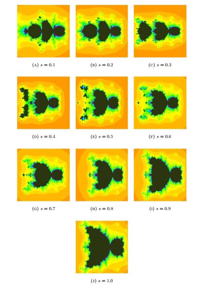
Examples of a quadratic Mandelbrot set, i.e., the set for \(Q_c(z) = z^2 + c\), in the \(S\) orbit with \(s\)-convexity are presented in Fig. 1. The common parameters used to generate the images were the following: \(K = 50\), \(\gamma = 0.7\), \(\delta = 0.2\). Whereas, the varying parameters were the following: (a) \(A = [-2, 0.3] \times [-1.2, 1.2]\), \(s = 0.1\), (b) \(A = [-2.4, 0.5] \times [-1.5, 1.5]\), \(s = 0.2\), (c) \(A = [-2.6, 0.5] \times [-1.8, 1.8]\), \(s = 0.3\), (d) \(A = [-3, 0.9] \times [-2, 2]\), \(s = 0.4\), (e) \(A = [-3.5, 0.9] \times [-2, 2]\), \(s = 0.5\), (f) \(A = [-4, 1] \times [-2.5, 2.5]\), \(s = 0.6\), (g) \(A = [-4.5, 1] \times [-2.7, 2.7]\), \(s = 0.7\), (h) \(A = [-6, 1] \times [-3, 3]\), \(s = 0.8\), (i) \(A = [-6, 1] \times [-3, 3]\), \(s = 0.9\), (j) \(A = [-6, 1] \times [-3, 3]\), \(s = 1.0\).

4.2. Mandelbrot sets for the cubic polynomial \(Q_{c}(z)=z^{3}+c\)

Examples of a cubic Mandelbrot set, i.e., the set for \(Q_c(z) = z^3 + c\), in the \(S\) orbit with \(s\)-convexity are presented in Fig. 2. The common parameters used to generate the images were the following: \(K = 50\), \(\gamma = 0.6\), \(\delta = 0.4\). Whereas, the varying parameters were the following: (a) \(A = [-0.7, 0.7] \times [-1, 1]\), \(s = 0.1\), (b) \(A = [-0.8, 0.8] \times [-1.3, 1.3]\), \(s = 0.2\), (c) \(A = [-1, 1] \times [-1.5, 1.5]\), \(s = 0.3\), (d) \(A = [-1, 1] \times [-2, 2]\), \(s = 0.4\), (e) \(A = [-1, 1] \times [-2, 2]\), \(s = 0.5\), (f) \(A = [-1, 1] \times [-2, 2]\), \(s = 0.6 ,(g), A = [-1, 1] \times [-2.2, 2.2]\), \(s = 0.7\), (h) \(A = [-1, 1] \times [-2.5, 2.5]\), \(s = 0.8\), (i) \(A = [-1, 1] \times [-2.5, 2.5]\), \(s = 0.9\), (j) \(A = [-1.5, 1.5] \times [-2.5, 2.5]\), \(s = 1.0\).

4.3. Mandelbrot sets for the polynomial \(Q_{c}(z)=z^{k+1}+c\), where \(k=3\)

Examples of the fourth order Mandelbrot set, i.e., the set for \(Q_c(z) = z^4 + c\), in the \(S\) orbit with \(s\)-convexity are presented in Fig. 3 . The common parameters used to generate the images were the following: \(K = 50\), \(\gamma = 0.5\), \(\delta = 0.3\). Whereas, the varying parameters were the following: (a) \(A = [-0.9, 0.7] \times [-0.7, 0.7]\), \(s = 0.1\), (b) \(A = [-1.1, 0.8] \times [-0.8, 0.8]\), \(s = 0.2\), (c) \(A = [-1.3, 1] \times [-0.9, 0.9]\), \(s = 0.3\), (d) \(A = [-1.4, 1] \times [-1.1, 1.1]\), \(s = 0.4\), (e) \(A = [-1.5, 1.1] \times [-1.3, 1.3]\), \(s = 0.5\), (f) \(A = [-1.7, 1.2] \times [-1.4, 1.4]\), \(s = 0.6\), (g) \(A = [-1.8, 1.3] \times [-1.5, 1.5]\), \(s = 0.7\), (h) \(A = [-1.8, 1.4] \times [-1.6, 1.6]\), \(s = 0.8\), (i) \(A = [-1.8, 1.5] \times [-1.6, 1.6]\), \(s = 0.9\), (j) \(A = [-1.8, 1.5] \times [-1.6, 1.6]\), \(s = 1.0\).

4.4. Julia sets for the quadratic polynomial \(Q_{c}(z)=z^{2}+c\)

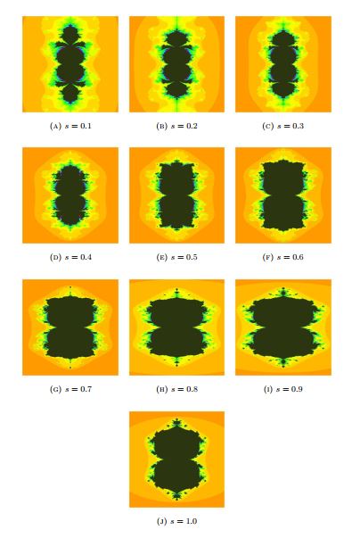
Examples of a quadratic Julia set, i.e., the set for \(Q_c(z) = z^2 + c\), in the \(S\) orbit with \(s\)-convexity are presented in Fig. 4. The common parameters used to generate the images were the following: \(c = -1.45 + 0.3\mathbf{i}\), \(K = 50\), \(\gamma = 0.3\), \(\delta = 0.5\). Whereas, the varying parameters were the following: (a) \(A = [-2.1, 1.3] \times [-1, 1]\), \(s = 0.1\), (b) \(A = [-2.5, 1.5] \times [-1.4, 1.4]\), \(s = 0.2\), (c) \(A = [-2.3, 1.5] \times [-1.4, 1.4]\), \(s = 0.3\), (d) \(A = [-2.5, 1.7] \times [-1.6, 1.6]\), \(s = 0.4\), (e) \(A = [-2.5, 1.7] \times [-1.8, 1.8]\), \(s = 0.5\), (f) \(A = [-2.5, 1.7] \times [-2, 2]\), \(s = 0.6\), (g) \(A = [-2.5, 1.8] \times [-2.3, 2.3]\), \(s = 0.7\), (h) \(A = [-2.5, 1.8] \times [-2.6, 2.6]\), \(s = 0.8\), (i) \(A = [-2.5, 1.8] \times [-2.9, 2.9]\), \(s = 0.9\), (j) \(A = [-2.8, 2.3] \times [-3.4, 3.4]\), \(s = 1.0\).

5. Conclusions

In this paper we proposed the use instead of a convex combination the \(s\)-convex combination in the \(S\)-iteration. Using this modified \(S\)-iteration we derived escape criteria for the polynomial function of the form \(z^{k+1} + c\), where \(c \in \mathbb{C}\) and \(k = 1, 2, \ldots\). Moreover, we presented some graphical examples of Mandelbrot and Julia sets generated using the escape time algorithm with the derived escape criteria. Very interesting changes in the Mandelbrot and Julia sets can be observed when \(s\) varies from low to high values. Because the \(s\)-convex combination is a generalization of the convex combination, thus the results presented in this paper are generalization of the results obtained by Kang et al. in [14].

In our further work we will try to derive the escape criteria in the \(S\)-iteration with \(s\)-convexity for functions of other classes than the polynomial one, e.g., trigonometric. Moreover, in the fixed point literature we can find many different iteration methods that can be used in the study of Julia and Mandelbrot sets. A review of explicit iterations and their dependencies can be found in [26].

Competing Interest

The authors declare no competing interest.

References

Mandelbrot, B. B. (1983). The fractal geometry of nature (Vol. 173). New York: WH freeman.[Google Scholor]
Dhurandhar, S. V., Bhavsar, V. C., & Gujar, U. G. (1993). Analysis of \(z\)-plane fractal images from \(z\leftarrow z^{\alpha}+ c\) for \(a< 0\). Computers & Graphics, 17(1), 89-94.
Lakhtakia, A., Varadan, V. V., Messier, R., & Varadan, V. K. (1987). On the symmetries of the Julia sets for the process \(z\leftarrow z^p+ c\). Journal of Physics A: Mathematical and General, 20(11), 3533.[Google Scholor]
Peherstorfer, F., & Stroh, C. (2001). Connectedness of Julia sets of rational functions. Computational Methods and Function Theory, 1(1), 61-79. [Google Scholor]
Domínguez, P., & Fagella, N. (2008, January). Residual Julia sets of rational and transcendental functions. In Transcendental dynamics and complex analysis (pp. 138-164). [Google Scholor]
Koss, L. (2016). Elliptic Functions with Disconnected Julia Sets. Int. J. Bifurcation Chaos, 26(6), 1650095 (2016) [10 pages].[Google Scholor]
Crowe, W. D., Hasson, R., Rippon, P. J., & Strain-Clark, P. E. D. (1989). On the structure of the Mandelbar set. Nonlinearity, 2(4), 541.[Google Scholor]
Dang, Y., Kauffman, L. H., & Sandin, D. J. (2002). Hypercomplex Iterations: Distance Estimation and Higher Dimensional Fractals (Vol. 1). World Scientific. ISBN: 978-981-02-3296-2 [Google Scholor]
Griffin, C. J., & Joshi, G. C. (1992). Octonionic Julia sets. Chaos, Solitons & Fractals, 2(1), 11-24.[Google Scholor]
Katunin, A. (2016, September). Analysis of 4D Hypercomplex Generalizations of Julia Sets. In International Conference on Computer Vision and Graphics (pp. 627-635). Springer, Cham. [Google Scholor]
Rani, M., & Kumar, V. (2004). Superior Julia set. Research in Mathematical Education, 8(4), 261-277.[Google Scholor]
Rani, M., & Kumar, V. (2004). Superior Mandelbrot set. Research in Mathematical Education, 8(4), 279-291.[Google Scholor]
Chauhan, Y. S., Rana, R., & Negi, A. (2010). New Julia sets of Ishikawa iterates. International Journal of Computer Applications, 7(13), 34-42.[Google Scholor]
Kang, S. M., Rafiq, A., Latif, A., Shahid, A. A., & Ali, F. (2016). Fractals through Modified Iteration Scheme. Filomat, 30(11), 3033-3046. [Google Scholor]
Kang, S. M., Rafiq, A., Latif, A., Shahid, A. A., & Kwun, Y. C. (2015). Tricorns and Multicorns of-Iteration Scheme. Journal of Function Spaces, Volume 2015, Article ID 417167, 7 pages. [Google Scholor]
Rani, M., & Chugh, R. (2014). Julia sets and Mandelbrot sets in Noor orbit. Applied Mathematics and Computation, 228, 615-631. [Google Scholor]
Pinheiro, M. R. (2008). S-convexity (Foundations for Analysis). Differ. Geom. Dyn. Syst, 10, 257-262.[Google Scholor]
Mishra, M. K., Ojha, D. B., & Sharma, D. (2011). Fixed point results in tricorn and multicorns of Ishikawa iteration and s-convexity. IJEST, 2(2), 157-160.[Google Scholor]
Mishra, M. K., & Ojha, D. B. Some Common Fixed Point Results In Relative Superior Julia Sets With Ishikawa Iteration And S-Convexity. IJAEST 2(2), 174 – 179 [Google Scholor]
Kang, S. M., Nazeer, W., Tanveer, M., & Shahid, A. A. (2015). New Fixed Point Results for Fractal Generation in Jungck Noor Orbit with-Convexity. Journal of Function Spaces, Volume 2015 (2015), Article ID 963016, 7 pages.[Google Scholor]
Nazeer, W., Kang, S. M., Tanveer, M., & Shahid, A. A. (2015). Fixed point results in the generation of Julia and Mandelbrot sets. Journal of Inequalities and Applications, 2015(1), 298.[Google Scholor]
Cho, S. Y., Shahid, A. A., Nazeer, W., & Kang, S. M. (2016). Fixed point results for fractal generation in Noor orbit and s-convexity. SpringerPlus, 5(1), 1843.[Google Scholor]
Barnsley, M. F. (1988). Fractals Everywhere, Acad. Press, New York.[Google Scholor]
Devaney, R. L. (1993). A First Course in Chaotic Dynamical Systems: Theory and Experiment., Avalon Publishing,CA 94608-1077 USA.[Google Scholor]
Agarwal, R. P., O Regan, D., & Sahu, D. R. (2007). Iterative construction of fixed points of nearly asymptotically nonexpansive mappings. Journal of Nonlinear and convex Analysis, 8(1), 61-79.[Google Scholor]
Gdawiec, K., & Kotarski, W. (2017). Polynomiography for the polynomial infinity norm via Kalantari’s formula and nonstandard iterations. Applied Mathematics and Computation, 307, 17-30.[Google Scholor]