In this paper, dynamics of a two-dimensional Fitzhugh-Nagumo model is discussed. The discrete-time model is obtained with the implementation of forward Euler’s scheme. We present the parametric conditions for local asymptotic stability of steady-states. It is shown that the two-dimensional discrete-time model undergoes period-doubling bifurcation and Neimark-Sacker bifurcation at its positive steady-state. Furthermore, in order to illustrate theoretical discussion some interesting numerical examples are presented.
where \(a_1\), \(b_1\) and \(c_1\) are positive constants. Using the forward Euler method to system (1), we get the discrete-time model as follows:
\begin{equation}\label{eq1}
\left(
\begin{array}{c}
x \\
y \\
\end{array}
\right)\to\left(
\begin{array}{c}
x+h c_1\left(x+y-\frac{x^3}{3}\right) \\
y-\frac{h}{c_1}\left(x-a_1+b_1y\right)\\
\end{array}
\right),
\end{equation}
(2)
where \(h>0\) is step size. For further biological relevance and dynamical analysis of some models that are very close to system (2),
we refer to [2,3, 4, 5, 6, 7, 8, 9, 10, 11, 12, 13, 14, 15 ], and references are therein.
We investigate the existence of equilibria for (2) and local asymptotic stability of these steady-states by implementing linearized stability analysis techniques. Also, Neimark-Sacker bifurcation and period-doubling bifurcation are discussed.
2. Existence of equilibria and stability
The steady-states of (2) satisfy the following system of algebraic equations:
If \(\Delta > 0\), then system (2) has three distinct equilibrium points.
If \(\Delta = 0\), then system (2) has a multiple equilibrium points.
If \(\Delta < 0\), then system (2) has a unique positive equilibrium point.
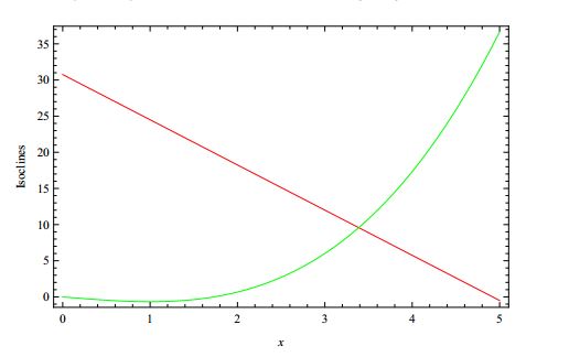
For \(a_1=4.92\) and \(b_1=0.16\), we have \(\Delta=-5.95649< 0\) and existence for unique positive equilibrium is depicted
in Figure 1.
Figure 1. For \(a_1=4.92\) and \(b_1=0.16\) existence of unique positive equilibrium for (2).
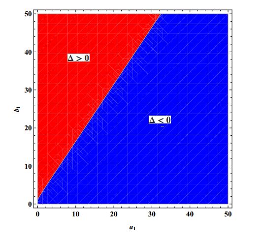
For \(a_1\in[0,50]\) and \(b_1\in[0,50]\), the region (blue) where \(\Delta0\)
are depicted in Figure 2.
Figure 2. Regions for existence of various equilibria.
Mathematically, we have the following conditions for negativity and positivity of \(\Delta\):
\(\Delta< 0\) if and only if \(0< b_1\le1\), or \(b_1>1\) and \(a_1>\frac{2}{3} \sqrt{\frac{-1+3 b_1-3b_1^2+b_1^3}{b_1}}\).
\(\Delta>0\) if and only if \(b_1>1\) and \(a_1< \frac{2}{3} \sqrt{\frac{-1+3 b_1-3b_1^2+b_1^3}{b_1}}\).
\(\Delta=0\) if and only if \(b_1>1\) and \(a_1=\frac{2}{3} \sqrt{\frac{-1+3 b_1-3b_1^2+b_1^3}{b_1}}\).
Now the Jacobian matrix of (2) evaluated at arbitrary equilibrium \((x,y)\) is given by:
$$
J(x,y):=\left(
\begin{array}{cc}
1+\left(h-h x^2\right) c_1 & h c_1 \\
-\frac{h}{c_1} & 1-\frac{h b_1}{c_1}
\end{array}
\right).
$$
Moreover, the characteristic polynomial of \(J(x,y)\) is given by:
\begin{equation}\label{ch}
\begin{split}
P(\lambda)&:=\lambda^2-\left(2-\frac{b_1 h}{c_1}+c_1 h \left(1-x^2\right)\right)\lambda\\
&+1+h \left(c_1+h-c_1 x^2\right)-
\frac{b_1 h \left(1+c_1 h \left(1-x^2\right)\right)}{c_1}.
\end{split}
\end{equation}
(5)
Theorem 2.1.
[16]
Assume that \(\Delta< 0\), then unique positive equilibrium \((x,y)\) has the following topological classification:
(i) \((x,y)\) is a sink if and only if
$$
\left|2-\frac{b_1 h}{c_1}+c_1 h \left(1-x^2\right)\right|< 2+h \left(c_1+h-c_1 x^2\right)-
\frac{b_1 h \left(1+c_1 h \left(1-x^2\right)\right)}{c_1}0,
$$
and
$$
\left|2-\frac{b_1 h}{c_1}+c_1 h \left(1-x^2\right)\right|>\left|2+h \left(c_1+h-c_1 x^2\right)-
\frac{b_1 h \left(1+c_1 h \left(1-x^2\right)\right)}{c_1}\right|.
$$
(iii) \((x,y)\) is a source if and only if
$$
\left|1+h \left(c_1+h-c_1 x^2\right)-
\frac{b_1 h \left(1+c_1 h \left(1-x^2\right)\right)}{c_1}\right|>1,
$$
and
$$
\left|2-\frac{b_1 h}{c_1}+c_1 h \left(1-x^2\right)\right|< \left|2+h \left(c_1+h-c_1 x^2\right)-
\frac{b_1 h \left(1+c_1 h \left(1-x^2\right)\right)}{c_1}\right|.
$$
(iv) \((x,y)\) is non-hyperbolic if and only if
$$
\left|2-\frac{b_1 h}{c_1}+c_1 h \left(1-x^2\right)\right|=\left|2+h \left(c_1+h-c_1 x^2\right)-
\frac{b_1 h \left(1+c_1 h \left(1-x^2\right)\right)}{c_1}\right|,
$$
or
$$
\left(c_1+h-c_1 x^2\right)-
\frac{b_1 \left(1+c_1 h \left(1-x^2\right)\right)}{c_1}=0
$$
and
$$
\left|2-\frac{b_1 h}{c_1}+c_1 h \left(1-x^2\right)\right|\le2.
$$
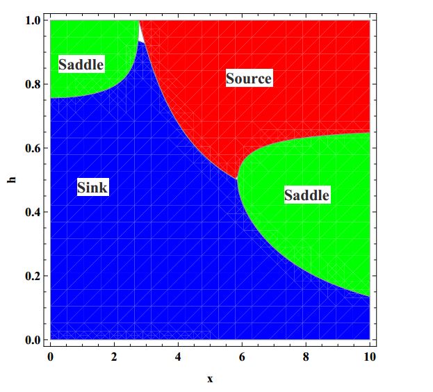
If we choose \(b_1=0.45\), \(c_1=0.15\), \(h\in[0,1]\) and \(x\in[0,10]\), then topological classification
for unique positive point of system (2) is shown in Figure 3.
Figure 3. Topological classification for positive equilibrium.
3. Bifurcation analysis
Studying bifurcation analysis for discrete-time models is a topic of great interest.
Recently, there are many articles have published for the investigation for period-doubling
and Neimark-Sacker bifurcations in discrete-time models [17, 18, 19, 20, 21, 22, 23].
In this section, we explore the parametric conditions under which system (2)
undergoes period-doubling and Neimark-Sacker bifurcations at its unique positive equilibrium point.
For this, first we discuss the emergence of period-doubling bifurcation at positive equilibrium
of system (2). Assume that \(P(-1)=0\), where \(P(\lambda)\) is defined in (5), then system
(2) undergoes period-doubling bifurcation as \(h\) varies in a small neighborhood of \(h_0\) defined by
$$
h_0:=\frac{b_1+\left(-1+x^2\right) c_1^2-\sqrt{-4 c_1^2+\left(b_1-\left(-1+x^2\right) c_1^2\right){}^2}}{\left(1+\left(-1+x^2\right) b_1\right) c_1},
$$
or
$$
h_0:=\frac{b_1+\left(-1+x^2\right) c_1^2+\sqrt{-4 c_1^2+\left(b_1-\left(-1+x^2\right) c_1^2\right){}^2}}{\left(1+\left(-1+x^2\right) b_1\right) c_1}.
$$
Secondly, we assume that
$$
\left(b_1+\left(-1+x^2\right) c_1^2\right){}^2 \left(-4 c_1^2+\left(b_1-\left(-1+x^2\right) c_1^2\right){}^2\right)< 0.
$$
Then system (2) undergoes Neimark-Sacker bifurcation as parameter \(h\) varies in a small neighborhood of \(h_1\) defined by:
$$
h_1:=\frac{b_1+\left(-1+x^2\right) c_1^2}{\left(1+\left(-1+x^2\right) b_1\right) c_1}.
$$
In order to verify aforementioned mathematical investigation for existence of period-doubling and Neimark-Sacker bifurcations,
we choose particular parametric values for system (2) as follows:
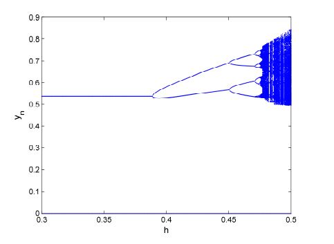
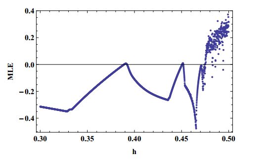
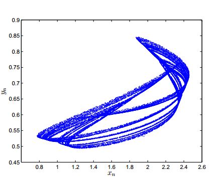
[Period-doubling bifurcation] Let \(a_1=2.6\), \(b_1=1.2\), \(c_1=1.9\) and \(h\in[0.3,0.5]\). In this case, system
(2) undergoes period-doubling bifurcation as \(h\) varies in a small neighborhood of \(h_0=0.39\). Moreover, the
bifurcation diagrams for period-doubling bifurcation are shown in Figure 4 and Figure 5. Moreover, maximum
Lyapunov exponents (MLE) are shown in Figure 6 and a chaotic attractor is depicted in Figure 7.
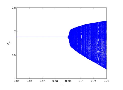
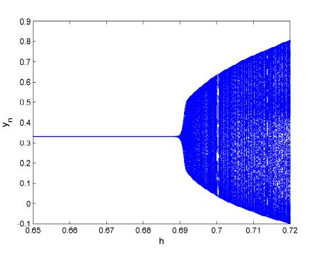
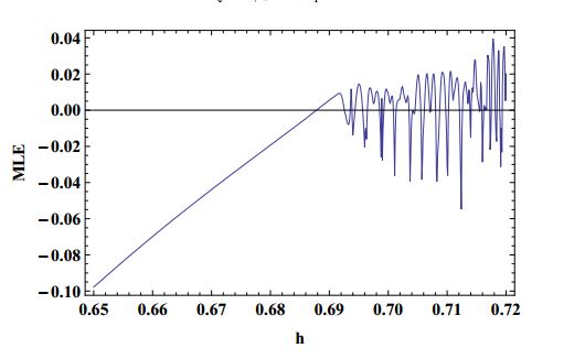
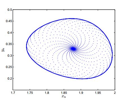
[Neimark-Sacker bifurcation] Taking \(a_1=2.7\), \(b_1=2.5\), \(c_1=0.95\) and \(h\in[0.65,0.72]\).
Then system (2) undergoes Neimark-Sacker bifurcation as \(h\) varies in a small neighborhood
of \(h_1=0.69\). The diagrams for Neimark-Sacker bifurcation are given in Figure 8 and Figure 9.
Furthermore, MLE are shown in Figure 10 and phase portrait at \(h=0.69\) is depicted in Figure 11.
Figure 4. Bifurcation diagram for \(x_n\).Figure 5. Bifurcation diagram for \(y_n\).Figure 6. Maximum Lyapunov exponents.Figure 7. A chaotic attractor at \(h=0.5\).Figure 8. Bifurcation diagram for \(x_n\).Figure 9. Bifurcation diagram for \(y_n\).Figure 10. Maximum Lyapunov exponents.Figure 11. Phase portrait at \(h=0.69\).
4. Conclusion
The qualitative behavior for a two-dimensional discrete-time Fitzhugh-Nagumo model is investigated.
Euler’s forward scheme is implemented to obtain the discrete counterpart of the continuous Fitzhugh-Nagumo model.
It is investigated that discrete-time model has rich dynamical behavior as compare to its continuous counterpart.
The topological classification for steady-state solutions is discussed. Furthermore, parametric conditions for
the existence of period-doubling bifurcation and Neimark-Sacker bifurcation are analyzed by taking \(h\) as bifurcation
parameter. At the end numerical simulations are provided to illustrate the theoretical discussion.
Competing Interests
The author(s) do not have any competing interests in the manuscript.
References
FitzHugh, R. (1961). Impulses and physiological state in theoretical models of nerve membrane. Biophysical Journal, 1(6), 445-467. [Google Scholor]
Hodgkin, A. L., & Huxley, A. F. (1952). A quantitive description of membrane current and its application to conduction and excitation in nerve. The Journal of Physiology, 117(4), 500-544.[Google Scholor]
Hindmarsh, J. L., & Rose, R. M. (1984). A model of neuronal bursting using three coupled first order differential equations. Biological Sciences, Proceedings of the Royal Society of London B, 221(1222), 87-102. [Google Scholor]
Buzzi, C., Llibre, J., & Medrado, J. (2015). Hopf and zero-Hopf bifurcations in the
Hindmarsh-Rose system. Nonlinear Dynamics, 83(3), 1549-1556. [Google Scholor]
Chay, T. R., & Keizer, J. (1985). Theory of the effect of extracellular potassium on oscillations in the pancreatic beta cell. Biophysical Journal, 48(5), 815-827. [Google Scholor]
Chay, T. R., & Rinzel, J. (1985). Bursting, beating and chaos in an excitable membrane model. Biophysical Journal, 47(3) 357-366. [Google Scholor]
Chay, T. R. (1985). Chaos in a three-variable model of an excitable cell. Physical Dynamics, 16(2), 233-242.[Google Scholor]
Chay, T. R. (1985). Glucose response to bursting-spiking pancreatic beta-cells by a barrier kinetic model. Biological Cybernetics, 52(5), 339-349. [Google Scholor]
Chen, S. S., Cheng, C. Y., & Rulin, Y. (2013). Application of a two-dimensional Hindmarsh-Rose type model for bifurcation analysis. International Journal of Bifurcation and Chaos, 23(3), 1350055. [Google Scholor]
Innocenti, G., Morelli, A., Genesio, R., & Torcini, A. (2007). Dynamical phases of the Hindmarsh-Rose neuronal model: Studies of the transition from bursting to spiking chaos. Chaos, 17(4), 043128. [Google Scholor]
Jing, Z. J., Chang, Y., & Guo, B. L. (2004). Bifurcation and chaos in discrete FitzHugh–Nagumo system. Chaos, Solitons and Fractals, 21(3), 701-720. [Google Scholor]
Liu, X. L., & Liu, S. Q. (2012). Codimension-two bifurcation analysis in two dimensional Hindmarsh-Rose model. Nonlinear Dynamics, 67(1), 847-857. [Google Scholor]
Lange, E., & Hasler, M. (2008). Predicting single spikes and spike patterns with the Hindmarsh-Rose model. Biological Cybernetics, 99: 349. [Google Scholor]
Li, B., & He, Z. (2014). Bifurcation and chaos in a two-dimensional discrete Hindmarsh-Rose model. Nonlinear Dynamics, 76(1), 697-715. [Google Scholor]
Rocsoreanu, C., Georgescu, A., & Giurgiteanu, N. (2000). FitzHugh-Nagumo model: Bifurcation and Dynamics. Springer, Dordrechts. ISBN 978-94-015-9548-3 [Google Scholor]
Kulenovi\'{c}, M. R. S., & Ladas, G. (2002). Dynamics of Second Order Rational Difference Equations: With
Open Problems and Conjectures. Chapman and Hall/CRC, New York. ISBN 9781584882756 [Google Scholor]
Din, Q. (2018). A novel chaos control strategy for discrete-time Brusselator models. Journal of Mathematical Chemistry. [Google Scholor]
Din, Q., & Hussain, M. (2018). Controlling chaos and Neimark-Sacker bifurcation in a host-parasitoid model.
Asian Journal of Control. [Google Scholor]
Din, Q., Elsadany, A. A., & Ibrahim, S. (2018). Bifurcation analysis and chaos control in a second-order rational difference equation. International Journal of Nonlinear Sciences and Numerical Simulation, 19(1), 53–68. [Google Scholor]
Din, Q. (2018). Bifurcation analysis and chaos control in discrete-time glycolysis models.
Journal of Mathematical Chemistry. 56(3): 904–931.[Google Scholor]
Din, Q., Donchev, T., & Kolev, D. (2018). Stability, Bifurcation Analysis and Chaos Control in Chlorine Dioxide-Iodine-Malonic Acid Reaction. MATCH-Communications in Mathematical and in Computer Chemistry, 79(3), 577–606. [Google Scholor]
Din, Q. (2018). Controlling chaos in a discrete-time prey-predator model with Allee effects.
International Journal of Dynamics and Control, 6(2), 858-872. [Google Scholor]
Din, Q. (2018). Qualitative analysis and chaos control in a density-dependent host-parasitoid system. International Journal of Dynamics and Control, 6(2), 778–798. [Google Scholor]