Open Journal of Mathematical Sciences

M-Polynomials and degree-based Topological Indices of Some Families of Convex Polytopes

Muhammad Riaz, Wei Gao\(^{1}\), Abdul Qudair Baig
Department of Mathematics and Statistics, The University of Lahore, Pakistan. (M.R)
School of Information Science and Technology,Yunnan Normal University, Kunming 650500, China. (W.G)
Department of Mathematics, The University of Lahore, Pakpattan Campus, Pakistan.(A.Q.B)

\(^{1}\)Corresponding Author: aowei@ynnu.edu.cn

Abstract

In this article, we compute closed forms of M-polynomial for three general classes of convex polytopes. From the M-polynomial, we derive degree-based topological indices such as first and second Zagreb indices, modified second Zagreb index, Symmetric division index, etc.

Keywords:

M-polynomial, degree-based topological index, convex polytope.

1. Introduction

A graph \(G(V,E)\) with vertex set \(V(G)\) and edge set \(E(G)\) are connected, if there exists a connection between any pair of vertices in \(G.\) The degree of a vertex is the number of vertices which are connected to that fixed vertex by the edges. In a chemical graph, the degree of any vertex is at most 4. The distance between two vertices \(u\) and \(v\) is denoted as \(d(u,v)=d_{G} (u,v)\) and is the length of shortest path between \(u\) and \(v\) in graph \(G.\) The number of vertices of \(G,\) adjacent to a given vertex \(v,\) is the ''degree'' of this vertex, and will be denoted by \(d_{v} \). The concept of degree in graph theory is closely related (but not identical) to the concept of valence in chemistry. For details on basics of graph theory, any standard text such as [1] can be of great help. Several algebraic polynomials have useful applications in chemistry such as Hosoya polynomial (also called Wiener polynomial) [2], which plays a vital role in determining distance-based topological indices. Among other algebraic polynomials, M-polynomial [3] introduced in 2015, plays the same role in determining closed form of many degree-based topological indices [4, 5, 6, 7, 8]. The main advantage of M-polynomial is the wealth of information that it contains about degree-based graph invariants.

Definition 1.1. [3] The M-polynomial of \textit{G} is defined as: \begin{equation*} M\left(G,x,y\right)=\sum _{\delta \le i\le j\le \Delta }m_{ij} \left(G\right)x^{i} y^{j} \end{equation*} where \(\delta ={\rm Min}\{ d_{v} |v\in {\rm V\; (G)}\} ,\) \(\Delta ={\rm Max}\{ d_{v} |v\in {\rm V\; (G)}\} ,\) and \(m_{ij} (G)\) is the edge \(vu\in E(G)\) such that \(\left\{d_{v} ,d_{u} \right\}=\left\{i,j\right\}.\)

The first topological index was introduced by Wiener [9] and it was named path number, which is now known as Wiener index. In chemical graph theory, this is the most studied molecular topological index due to its wide applications; see for details in [10, 11]. Rendić index, [12] denoted by \(R_{-1/2} (G)\) and introduced by Milan Rendić in 1975 is also one of the oldest topological index. The Rendić index is defined as \begin{equation*} R_{-1/2} (G)=\sum _{uv\in E(G)}\frac{1}{\sqrt{d_{u} d_{v} } }. \end{equation*} In 1998, working independently, Bollobás and Erdös, [13] and Amic et al. [14] proposed the generalized Rendić index which has been studied extensively by both chemists and mathematicians [15]. Many mathematical properties have been discussed [16]. For a detailed survey we refer the book [17].
The general Rendić index is defined as: \begin{equation*} R_{\alpha } (G)=\sum _{uv\in E(G)}\frac{1}{(d_{u} d_{v} )^{\alpha } }, \end{equation*} and the inverse Rendić index is defined as \(RR_{\alpha } (G)=\sum _{uv\in E(G)}(d_{u} d_{v} )^{\alpha }. \)
Obviously \(R_{-1/2} (G)\) is the particular case of \(R_{\alpha } (G)\) when \(\alpha =-\frac{1}{2} \).
The Rendić index is the most popular most often applied and most studied among all other topological indices. Many papers and books such as [17, 18, 20] are written on this topological index. Rendić himself wrote two reviews on his Rendić index [21, 22] and there are three more reviews [23, 24, 25]. The suitability of the Rendić index for drug design was immediately recognized, and eventually the index was used for this purpose on countless occasions. The physical reason for the success of such a simple graph invariant is still an enigma, although several more-or-less plausible explanations were offered.
Gutman and Trinajsti\'c introduced first Zagreb index and second Zagreb index, which are defined as: \(M_{1} (G)=\sum _{uv\in E(G)}(d_{u} +d_{v} ) \) and \(M_{2} (G)=\sum _{uv\in E(G)}(d_{u} \times d_{v} ) \) respectively. The second modified Zagreb index is defined as: \begin{equation*} ^{m} M_{2} \left(G\right){\rm \; }=\sum _{uv\in E(G)}\frac{1}{d(u)d(v)} . \end{equation*} For details about these indices we offer [26, 27, 28, 29, 30] for the readers.
The Symmetric division index is defined as: \begin{equation*}{\rm SDD}\left({\rm G}\right){\rm \; }=\sum _{uv\in E(G)}\left\{\frac{\min (d_{u} ,d_{v} )}{\max (d_{u} ,d_{v} )} +\frac{\max (d_{u} ,d_{v} )}{\min (d_{u} ,d_{v} )} \right\}. \end{equation*} Another variant of Rendić index is the harmonic index defined as: \begin{equation*}H(G)=\sum _{vu\in E(G)}\frac{2}{d_{u} +d_{v} } . \end{equation*} The Inverse sum index is defined as: \begin{equation*} I(G)=\sum _{vu\in E(G)}\frac{d_{u} d_{v} }{d_{u} +d_{v} } . \end{equation*} The augmented Zagreb index is defined as: \begin{equation*} A(G)=\sum _{vu\in E(G)}\left\{\frac{d_{u} d_{v} }{d_{u} +d_{v} -2} \right\}^{3} , \end{equation*} and it is useful for computing heat of formation of alkanes [31, 32]. The following Table 1 relates some well-known degree-based topological indices with M-polynoimal [3].
Table 1. Derivation of some degree-based topological indices from M-polynomial.
Topological Index Derivation from \(M(G;x,y)\)
First Zagreb \(\left(D_{x} +D_{y} \right)(M(G;x,y))_{x=y=1} \)
Second Zagreb \(\left(D_{x} D_{y} \right)(M(G;x,y))_{x=y=1} \)
Second Modified Zagreb \(\left(S_{x} S_{y} \right)(M(G;x,y))_{x=y=1} \)
Rendić Index \(\left(D_{x}^{\alpha } D_{y}^{\alpha } \right)(M(G;x,y))_{x=y=1} \)
Inverse Rendić Index \(\left(S_{x}^{\alpha } S_{y}^{\alpha } \right)(M(G;x,y))_{x=y=1} \)
Symmetric Division Index \(\left(D_{x} S_{y} +S_{x} D_{y} \right)(M(G;x,y))_{x=y=1} \)
Harmonic Index \(2S_{x} J(M(G;x,y))_{x=1} \)
Inverse sum Index \(S_{x} JD_{x} D_{y} (M(G;x,y))_{x=1} \)
Augmented Zagreb Index \(S_{x} ^{3} Q_{-2} JD_{x} ^{3} D_{y} ^{3} (M(G;x,y))_{x=1} \)
where \[\begin{array}{l} {D_{x} =x\frac{\partial (f\left(x,y\right)}{\partial x} ,\; D_{y} =y\frac{\partial (f\left(x,y\right)}{\partial y} ,\; S_{x} =\mathop{\smallint }\limits_{0}^{x} \frac{f\left(t,y\right)}{t} dt,S_{y} =\mathop{\smallint }\limits_{0}^{y} \frac{f\left(x,t\right)}{t} dt\; ,}\\{\; J\left(f\left(x,y\right)\right)=f\left(x,x\right),\; } {Q_{\alpha } \left(f\left(x,y\right)\right)=x^{\alpha } f\left(x,y\right).} \end{array}\]

2. Main Results

In this section we give our main results.

2.1. Computational aspects of Convex Polytopes \(T_{n} \)

The graph of convex polytope \(T_{n} \) can be obtained from the graph of convex polytope \(Q_{n} \) by adding new edges. It consists of three-sided faces, five-sided faces and \(n\)-sided faces.
\(a_{i+1} b_{i} ,\) \textit{i.e.,} \(V\left(T_{n} \right)=V\left(Q_{n} \right)\)and \(V\left(T_{n} \right)=V\left(Q_{n} \right)\cup \left\{a_{i+1} b_{i} :{\rm \; \; \; }1\le i\le n\right\}\)as shown in figure 1.

Figure 2. Graph of Convex poltyope \(T_{6} \).

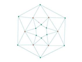
Theorem 2.1. Assume we have a convex polytope \(T_{n}\), then the M-Polynomial of \(T_{n}\) is \begin{equation*} M\left(T_{n} ;x,y\right)=2nx^{3} y^{3} +2nx^{3} y^{6} +nx^{4} y^{4} +2nx^{4} y^{6} +nx^{6} y^{6}. \end{equation*}

Proof. Let \(G=T_{n}\) be a convex polytope. It is easy to see form Figure 1 that \begin{equation*} \left|V\left(T_{n} \right)\right|=4n, \end{equation*} \begin{equation*} \left|E\left(T_{n} \right)\right|=8n. \end{equation*} The vertex set of \(S_{n} \) has two partitions: \begin{equation*} V_{1} (T_{n} )=\left\{u\in V(T_{n} ):{\rm \; \; \; }d_{u} =3\right\}, \end{equation*} \begin{equation*} V_{2} (T_{n} )=\left\{u\in V(T_{n} ):{\rm \; \; \; }d_{u} =4\right\},\end{equation*} \begin{equation*}V_{4} (T_{n} )=\left\{u\in V(T_{n} ):{\rm \; \; \; }d_{u} =6\right\}, \end{equation*} such that \begin{equation*} \left|V_{1} (T_{n} )\right|=2n,\left|V_{2} (T_{n} )\right|=n,\left|V_{3} (T_{n} )\right|=n, \end{equation*} The edge set of \(T_{n} \) has three partitions: \begin{equation*}E_{1} (T_{n} )=\left\{e=uv\in E(T_{n} ):{\rm \; \; \; }d_{u} =d_{v} =3\right\},\end{equation*} \begin{equation*}E_{2} (T_{n} )=\left\{e=uv\in E(T_{n} ):{\rm \; \; \; }d_{u} =3,d_{v} =6\right\},\end{equation*} \begin{equation*}E_{3} (T_{n} )=\left\{e=uv\in E(S_{n} ):{\rm \; \; \; }d_{u} =d_{v} =4\right\},\end{equation*} \begin{equation*}E_{4} (T_{n} )=\left\{e=uv\in E(T_{n} ):{\rm \; \; \; }d_{u} =4,d_{v} =6\right\},\end{equation*} \begin{equation*}E_{5} (T_{n} )=\left\{e=uv\in E(T_{n} ):{\rm \; \; \; }d_{u} =d_{v} =6\right\}, \end{equation*} From Figure 1, \begin{equation*} \left|E_{1} (T_{n} )\right|=2n,\left|E_{2} (T_{n} )\right|=2n,\left|E_{3} (T_{n} )\right|=n,\left|E_{4} (T_{n} )\right|=2n,\left|E_{5} (T_{n} )\right|=n, \end{equation*} From the definition of the M-polynomial \begin{align*} M\left(T_{n} ;x\; ,y\right)&=\mathop{\sum }\limits_{i\le j} m_{ij} \left(T_{n} \right)x^{i} y^{j} \nonumber \& =\mathop{\sum }\limits_{3\le 3} m_{33} \left(T_{n} \right)x^{3} y^{3} +\mathop{\sum }\limits_{3\le 6} m_{36} \left(T_{n} \right)x^{3} y^{6} +\mathop{\sum }\limits_{4\le 4} m_{44} \left(T_{n} \right)x^{4} y^{4} \nonumber\& +\mathop{\sum }\limits_{4\le 6} m_{46} \left(T_{n} \right)x^{4} y^{6} +\mathop{\sum }\limits_{6\le 6} m_{66} \left(T_{n} \right)x^{6} y^{6} \nonumber\& =\mathop{\sum }\limits_{uv\in E_{1} } m_{33} \left(T_{n} \right)x^{3} y^{3} +\mathop{\sum }\limits_{uv\in E_{2} } m_{36} \left(T_{n} \right)x^{3} y^{6} +\mathop{\sum }\limits_{uv\in E_{3} } m_{44} \left(T_{n} \right)x^{4} y^{4} \nonumber\& +\mathop{\sum }\limits_{uv\in E_{4} } m_{46} \left(T_{n} \right)x^{4} y^{6} +\mathop{\sum }\limits_{uv\in E_{5} } m_{66} \left(T_{n} \right)x^{6} y^{6} \nonumber\& =\left|E_{1} \right|x^{3} y^{3} +\left|E_{2} \right|x^{3} y^{6} +\left|E_{3} \right|x^{4} y^{4} +\left|E_{4} \right|x^{4} y^{6} +\left|E_{5} \right|x^{6} y^{6} \nonumber\& =2nx^{3} y^{3} +2nx^{3} y^{6} +nx^{4} y^{4} +2nx^{4} y^{6} +nx^{6} y^{6} . \end{align*}

Now we compute some degree-based topological indices of double antiprism from this M-polynomial.

Proposition 2.2. Let \(T_{n} \) be the double antiprism, then

  1. \(M_{1} (T_{n} )=70n.\)
  2. \(M_{2} (T_{n} )=154n\)
  3. \({}^{m} M_{2} (T_{n} )=\, \frac{73}{144} n.\)
  4. \(R_{\alpha } \left(T_{n} \right)=2\times 9^{\alpha } n+2\times 18^{\alpha } n+16^{\alpha } n+2\times 24^{\alpha } n+36^{\alpha } n.\)
  5. \(RR_{\alpha } \left(T_{n} \right)=\frac{2n}{9^{\alpha } } +\frac{2n}{16^{\alpha } } +\frac{n}{16^{\alpha } } +\frac{2n}{24^{\alpha } } +\frac{n}{36^{\alpha } } .\)
  6. \(SSD(T_{n} )=\frac{52}{3} n.\)
  7. \(H\left(T_{n} \right)=\frac{98}{45} n.\)
  8. \(I(T_{n} )=\frac{84}{5} n.\)
  9. \(A(T_{n} )==\frac{6534785489}{37044000} n.\)

Proof. Let \begin{equation*} M\left(T_{n} ;x,y\right)=f(x,y)=2nx^{3} y^{3} +2nx^{3} y^{6} +nx^{4} y^{4} +2nx^{4} y^{6} +nx^{6} y^{6} \end{equation*} Then \begin{equation*} D_{x} \left(f(x,y)\right)=6nx^{3} y^{3} +6nx^{3} y^{6} +4nx^{4} y^{4} +8nx^{4} y^{6} +6nx^{6} y^{6} ,\end{equation*} \begin{equation*}D_{y} \left(f(x,y)\right)=6nx^{3} y^{3} +12nx^{3} y^{6} +4nx^{4} y^{4} +12nx^{4} y^{6} +6nx^{6} y^{6} ,\end{equation*} \begin{equation*}\left(D_{y} D_{x} \right)\left(f(x,y)\right)=18nx^{3} y^{3} +36nx^{3} y^{6} +16nx^{4} y^{4} +48nx^{4} y^{6} +36nx^{6} y^{6} ,\end{equation*} \begin{equation*}S_{x} S_{y} (f(x,y))=\frac{2}{9} nx^{3} y^{3} +\frac{1}{9} nx^{3} y^{6} +\frac{1}{16} nx^{4} y^{4} +\frac{1}{12} nx^{4} y^{6} +\frac{1}{36} nx^{6} y^{6} ,\end{equation*} \begin{equation*}D_{x} ^{\alpha } D_{y} ^{\alpha } (f(x,y))=2\times 9^{\alpha } nx^{3} y^{3} +2\times 18^{\alpha } nx^{3} y^{6} +16^{\alpha } nx^{4} y^{4} +2\times 24^{\alpha } nx^{4} y^{6} +36^{\alpha } nx^{6} y^{6} ,\end{equation*} \begin{equation*}S_{x} ^{\alpha } S_{y} ^{\alpha } (f(x,y))=\frac{2n}{9^{\alpha } } x^{3} y^{3} +\frac{2n}{16^{\alpha } } x^{3} y^{6} +\frac{n}{16^{\alpha } } x^{4} y^{4} +\frac{2n}{24^{\alpha } } x^{4} y^{6} +\frac{n}{36^{\alpha } } x^{6} y^{6} ,\end{equation*} \begin{equation*}S_{y} D_{x} \left(f(x,y)\right)=2nx^{3} y^{3} +nx^{3} y^{6} +nx^{4} y^{4} +\frac{4n}{3} x^{4} y^{6} +nx^{6} y^{6} ,\end{equation*} \begin{equation*}S_{x} D_{y} \left(f(x,y)\right)=2nx^{3} y^{3} +4nx^{3} y^{6} +nx^{4} y^{4} +3nx^{4} y^{6} +nx^{6} y^{6} ,\end{equation*} \begin{equation*}S_{x} Jf(x,y)=\frac{n}{3} x^{6} +\frac{n}{4} x^{8} +\frac{2n}{9} x^{9} +\frac{n}{5} x^{10} +\frac{n}{12} x^{12} ,\end{equation*} \begin{equation*}S_{x} JD_{x} D_{y} \left(f(x,y)\right)==3nx^{6} +2nx^{8} +4nx^{9} +\frac{24}{5} nx^{10} +3nx^{12} ,\end{equation*} \begin{equation*}S_{x} ^{3} Q_{-2} JD_{x} ^{3} D_{y} ^{3} f(x,y)=\frac{1458}{64} nx^{4} +\frac{4096}{216} nx^{6} +\frac{11664}{343} nx^{7} +\frac{27648}{512} nx^{8} +\frac{46656}{1000} nx^{10} .\end{equation*} Now from Table 1

  1. \(M_{1} \left(T_{n} \right)=\left. \left(D_{x} +D_{y} \right)(f(x,y))\right|_{x=y=1} =70n.\)
  2. \(M_{2} \left(T_{n} \right)=\left. D_{x} D_{y} (f(x,y))\right|_{x=y=1} =154n.\)
  3. \({}^{m} M_{2} \left(T_{n} \right)=\left. S_{x} S_{y} (f(x,y))\right|_{x=y=1} =\frac{73}{144} n.\)
  4. \(R_{\alpha } \left(T_{n} \right)=\left. D_{x}^{\alpha } D_{y}^{\alpha } (f(x,y))\right|_{x=y=1} =2\times 9^{\alpha } n+2\times 18^{\alpha } n+16^{\alpha } n+2\times 24^{\alpha } n+36^{\alpha } n.\)
  5. \(RR_{\alpha } \left(T_{n} \right)=\left. S_{x}^{\alpha } S_{y}^{\alpha } (f(x,y))\right|_{x=y=1} =\frac{2n}{9^{\alpha } } +\frac{2n}{16^{\alpha } } +\frac{n}{16^{\alpha } } +\frac{2n}{24^{\alpha } } +\frac{n}{36^{\alpha } } \).
  6. \(SSD\left(T_{n} \right)=\left. \left(S_{y} D_{x} +S_{x} D_{y} \right)\left(f(x,y)\right)\right|_{x=y=1} =\frac{52}{3} n.\)
  7. \(H\left(T_{n} \right)=2S_{x} J\left(f(x,y)\right)|_{x=1} =\frac{98}{45} n.\)
  8. \(I\left(T_{n} \right)=S_{x} JD_{x} D_{y} \left(f(x,y)\right)_{x=1} =\frac{84}{5} n.\)
  9. \(A\left(T_{n} \right)=\left. S_{x} ^{3} Q_{-2} JD_{x} ^{3} D_{y} ^{3} \left(f(x,y)\right)\right|_{x=1} =\frac{6534785489}{37044000} n.\)

2.2. Computational aspects of Convex Polytopes \(A_{n}\)

The graph of convex polytope (double antiprism) \(A_{n}\) can be obtained from the graph of convex polytope \(R_{n}\) Rn by adding new edges \(b_{i+1} c_{i} ,\) i.e., \(V\left(A_{n} \right)=V\left(R_{n} \right)\(and \)V\left(A_{n} \right)=V\left(R_{n} \right)\cup \left\{b_{i+1} c_{i} :{\rm \; \; \; 1}\le {\rm i}\le {\rm n}\right\}\) as shown in Figure 2.

Figure 3. Graph of double antiprism \(A_{6} \).

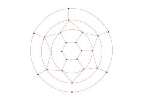
Theorem 2.3. Let \(A_{n}\) be the double antiprism, then the M-Polynomial of \(A_{n}\) is \begin{equation*} M\left(A_{n} \; ,\; x,y\right)=2nx^{4} y^{4} +4nx^{4} y^{6} +nx^{6} y^{6} \end{equation*}

Proof. Let \(G=A_{n}\) is double antiprism. It is easy to see form figure 2 that \begin{equation*} \left|V\left(A_{n} \right)\right|=3n, \end{equation*} \begin{equation*} \left|E\left(A_{n} \right)\right|=7n. \end{equation*} The vertex set of \(A_{n}\) has two partitions: \begin{equation*}V_{1} (A_{n} )=\left\{u\in V(A_{n} ):{\rm \; \; \; }d_{u} =4\right\}, \end{equation*} \begin{equation*} V_{2} (A_{n} )=\left\{u\in V(A_{n} ):{\rm \; \; \; }d_{u} =6\right\}, \end{equation*} such that \begin{equation*} \left|V_{1} (A_{n} )\right|=2n,\left|V_{2} (A_{n} )\right|=n. \end{equation*} The edge set of \(A_{n} \) has three partitions: \begin{equation*}E_{1} (A_{n} )=\left\{e=uv\in E(A_{n} ):{\rm \; \; \; }d_{u} =d_{v} =4\right\},\end{equation*} \begin{equation*}E_{2} (A_{n} )=\left\{e=uv\in E(A_{n} ):{\rm \; \; \; }d_{u} =4,d_{v} =6\right\},\end{equation*} \begin{equation*}E_{3} (A_{n} )=\left\{e=uv\in E(A_{n} ):{\rm \; \; \; }d_{u} =d_{v} =6\right\},\end{equation*} From Figure 2, \begin{equation*} \left|E_{1} (A_{n} )\right|=2n,\left|E_{2} (A_{n} )\right|=4n,\left|E_{3} (A_{n} )\right|=n, \end{equation*} Now from the definition of the M-polynomial \begin{align*} M\left(A_{n} ,\; x\; ,y\right)&=\mathop{\sum }\limits_{i\le j} m_{ij} \left(A_{n} \right)x^{i} y^{j} \nonumber \\ &=\mathop{\sum }\limits_{4\le 4} m_{44} \left(A_{n} \right)x^{4} y^{4} +\mathop{\sum }\limits_{4\le 6} m_{46} \left(A_{n} \right)x^{4} y^{6} {\rm \; }+\mathop{\sum }\limits_{5\le 5} m_{66} \left(A_{n} \right)x^{6} y^{6} \nonumber \\ &=\mathop{\sum }\limits_{uv\in E_{1} } m_{44} \left(A_{n} \right)x^{4} y^{4} +\mathop{\sum }\limits_{uv\in E_{2} } m_{46} \left(A_{n} \right)x^{4} y^{6} +\mathop{\sum }\limits_{uv\in E_{3} } m_{66} \left(A_{n} \right)x^{6} y^{6} \nonumber \\ &=\left|E_{1} \right|x^{4} y^{4} +\left|E_{2} \right|x^{4} y^{6} +\left|E_{3} \right|x^{6} y^{6} \nonumber \\ &=2nx^{4} y^{4} +4nx^{4} y^{6} +nx^{6} y^{6}. \end{align*}

Now we compute some degree-based topologcal indices of double antiprism from this M-polynomial.

Proposition 2.4. Let \(A_{n}\) be the double antiprism, then

  1. \(M_{1} (A_{n} )={\rm 68n}.\)
  2. \(M_{2} (A_{n} )=\frac{23}{72} n.\)
  3. \({}^{m} M_{2} (A_{n} )=\frac{23}{72} n.\)
  4. \(R_{\alpha } \left(A_{n} \right)=n(4\times 24^{\alpha } +36^{\alpha } +2\times 16^{\alpha } ).\)
  5. \(RR_{\alpha } \left(A_{n} \right)=n\left(\frac{2}{16^{\alpha } } +\frac{4}{24^{\alpha } } +\frac{1}{36^{\alpha } } \right).\)
  6. \(SSD(A_{n} )=\frac{44}{3} n.\)
  7. \(H\left(A_{n} \right)=\frac{11}{15} n.\)
  8. \(I(A_{n} )=\frac{83}{5} n.\)
  9. \(A(A_{n} )=\frac{649964}{3375} n.\)

2.3. Computational aspects of Convex Polytopes \(S_{n}\)

The graph of convex polytope (double antiprism) \(S_{n}\) can be obtained from the graph of convex polytope \(Q_{n}\) by adding new edges \(c_{i} c_{i+1} ,\) i.e., \(V\left(S_{n} \right)=V\left(Q_{n} \right)\) and \(V\left(S_{n} \right)=V\left(Q_{n} \right)\cup \left\{c_{i} c_{i+1} :{\rm \; \; \; 1}\le {\rm i}\le {\rm n}\right\}\) as shown in Figure 3.

Figure 3. Graph of double antiprism \(S_{6} \).

Theorem 2.5. Let \(S_{n}\) be the double antiprism, then the M-Polynomial of \(S_{n}\) is \begin{equation*} M\left(S_{n} ;\; x,y\right)=2nx^{3} y^{3} +2nx^{3} y^{5} +4nx^{5} y^{5} . \end{equation*}

Proof. Let \(G=S_{n}\) be the double antiprism. It is easy to see form Figure 3 that \begin{align*} \left|V\left(S_{n} \right)\right|&=4n, \\ \left|E\left(S_{n} \right)\right|&=8n. \end{align*} The vertex set of \(S_{n}\) has two partitions: \begin{align*} & V_{1} (S_{n} )=\left\{u\in V(S_{n} ):{\rm \; \; \; }d_{u} =3\right\}, \& V_{2} (S_{n} )=\left\{u\in V(S_{n} ):{\rm \; \; \; }d_{u} =5\right\}, \end{align*} such that \begin{align*} \left|V_{1} (S_{n} )\right|=2n,\left|V_{2} (S_{n} )\right|=2n. \end{align*} The edge set of \(A_{n}\) has three partitions: \begin{align*} & E_{1} (S_{n} )=\left\{e=uv\in E(S_{n} ):{\rm \; \; \; }d_{u} =d_{v} =3\right\},\& E_{2} (S_{n} )=\left\{e=uv\in E(S_{n} ):{\rm \; \; \; }d_{u} =3,d_{v} =5\right\},\& E_{3} (S_{n} )=\left\{e=uv\in E(S_{n} ):{\rm \; \; \; }d_{u} =d_{v} =5\right\}, \end{align*} From Figure 3, \begin{align*} \left|E_{1} (S_{n} )\right|=2n,\left|E_{2} (S_{n} )\right|=2n,\left|E_{3} (S_{n} )\right|=4n, \end{align*} Now from the definition of the M-polynomial \begin{align*} M\left(S_{n} ;x\; ,y\right)&=\mathop{\sum }\limits_{i\le j} m_{ij} \left(S_{n} \right)x^{i} y^{j}\nonumber \& =\mathop{\sum }\limits_{uv\in E_{1} } m_{33} \left(S_{n} \right)x^{3} y^{3} +\mathop{\sum }\limits_{uv\in E_{2} } m_{35} \left(S_{n} \right)x^{3} y^{5} +\mathop{\sum }\limits_{uv\in E_{3} } m_{55} \left(S_{n} \right)x^{5} y^{5} \nonumber \& =\left|E_{1} \right|x^{3} y^{3} +\left|E_{2} \right|x^{3} y^{5} +\left|E_{3} \right|x^{5} y^{5} \nonumber \& =2nx^{3} y^{3} +2nx^{3} y^{5} +4nx^{5} y^{5} . \end{align*}

Now we compute some degree-based topologcal indices of double antiprism from this M-polynomial.

Proposition 2.6. Let \(A_{n}\) be the double antiprism, then

  1. \(M_{1} (S_{n} )=68n.\)
  2. \(M_{2} (S_{n} )=148n.\)
  3. \({}^{m} M_{2} (S_{n} )=\frac{116}{225} n.\)
  4. \(R_{\alpha } \left(S_{n} \right)=2n(9^{\alpha } +15^{\alpha } +2\times 25^{\alpha } ).\)
  5. \(RR_{\alpha } \left(S_{n} \right)=2n\left(\frac{1}{9^{\alpha } } +\frac{1}{15^{\alpha } } +\frac{2}{25^{\alpha } } \right).\)
  6. \(SSD(S_{n} )=\frac{248}{15} n.\)
  7. \(H\left(S_{n} \right)=\frac{59}{60} n.\)
  8. \(I(S_{n} )=\frac{67}{4} n.\)
  9. \(A(S_{n} )=\frac{22541}{128} n.\)

3. Conclusions and Discussions

We computed closed forms of M-polynomial of three general classes of convex polytopes at first. Then we derived as many as nine degree-based topological indices such as first and second Zagreb indices, modified second Zagreb index, Symmetric division index, Augmented Zagreb index, Inverse-sum index etc.

Competing Interest

The authors declare no competing interest.

References

  1. Brückler, F. M., Došlic, T., Graovac, A., & Gutman, I. (2011). On a class of distance-based molecular structure descriptors. Chemical physics letters, 503(4-6), 336-338. [Google Scholor]
  2. Gutman, I. (1993). Some properties of the Wiener polynomial. Graph Theory Notes New York, 25, 13-18. [Google Scholor]
  3. Deutsch, E., & Klavžar, S. (2015). M-polynomial and degree-based topological indices. Iranian Journal of Mathematical Chemistry, 6(2), 93-102.[Google Scholor]
  4. Munir, M., Nazeer, W., Rafique, S., & Kang, S. M. (2016). M-polynomial and related topological indices of Nanostar dendrimers. Symmetry, 8(9), 97.[Google Scholor]
  5. Munir, M., Nazeer, W., Rafique, S., & Kang, S. M. (2016). M-polynomial and related topological indices of Nanostar dendrimers. Symmetry, 8(9), 97.[Google Scholor]
  6. Munir, M., Nazeer, W., Rafique, S., & Kang, S. M. (2016). M-polynomial and degree-based topological indices of polyhex nanotubes. Symmetry, 8(12), 149.[Google Scholor]
  7. Munir, M., Nazeer, W., Rafique, S., Nizami, A. R., & Kang, S. M. (2016). Some computational aspects of triangular Boron nanotubes. [Google Scholor]
  8. Munir, M., Nazeer, W., Shahzadi, Z., & Kang, S. M. (2016). Some invariants of circulant graphs. Symmetry, 8(11), 134. [Google Scholor]
  9. Wiener, H. (1947). Structural determination of paraffin boiling points. Journal of the American Chemical Society, 69(1), 17-20.[Google Scholor]
  10. Dobrynin, A. A., Entringer, R., & Gutman, I. (2001). Wiener index of trees: theory and applications. Acta Applicandae Mathematica, 66(3), 211-249. [Google Scholor]
  11. Gutman, I. & Polansky, O. E. (1986). Mathematical Concepts in Organic Chemistry. Springer-Verlag New York, USA. [Google Scholor]
  12. Randic, M. (1975). Characterization of molecular branching. Journal of the American Chemical Society, 97(23), 6609-6615. [Google Scholor]
  13. Bollobás, B., & Erdös, P. (1998). Graphs of extremal weights. Ars Combinatoria, 50, 225-233. [Google Scholor]
  14. Amić, D., Bešlo, D., Lučić, B., Nikolić, S., & Trinajstić, N. (1998). The vertex-connectivity index revisited. Journal of chemical information and computer sciences, 38(5), 819-822. [Google Scholor]
  15. Hu, Y., Li, X., Shi, Y., Xu, T., & Gutman, I. (2005). On molecular graphs with smallest and greatest zeroth-order general Randic index. MATCH Commun. Math. Comput. Chem, 54(2), 425-434. [Google Scholor]
  16. Caporossi, G., Gutman, I., Hansen, P., & Pavlovic, L. (2003). Graphs with maximum connectivity index. Computational Biology and Chemistry, 27(1), 85-90. [Google Scholor]
  17. Li, X., & Gutman, I. (2006). Mathematical Chemistry Monographs No. 1. University of Kragujevac, Kragujevac, Macedonia. [Google Scholor]
  18. Kier, L. B., & Hall, L. H. (1976). Molecular Connectivity in Chemistry and Drug Research Academic. New York.[Google Scholor]
  19. Kier, L. B., & Hall, L. H. (1986). Molecular connectivity in structure-activity analysis. Wiley, New York.[Google Scholor]
  20. Li, X., & Gutman, I. (2006). Mathematical aspects of Randic-type molecular structure descriptors. Math. Chem. Monographs, (1).[Google Scholor]
  21. Gutman, I. & Furtula, B. (2008). Recent Results in the Theory of Randic Index. University of Kragujevac, Kragujevac, Macedonia.
  22. Randic, M. (2008). On history of the Randic index and emerging hostility toward chemical graph theory. MATCH Commun. Math. Comput. Chem, 59, 5-124. [Google Scholor]
  23. Randic, M. (2001). The connectivity index 25 years after. Journal of Molecular Graphics and Modelling, 20(1), 19-35.[Google Scholor]
  24. Li, X., & Shi, Y. (2008). A survey on the Randic index. MATCH Commun. Math. Comput. Chem, 59(1), 127-156. [Google Scholor]
  25. Li, X., Shi, Y., & Wang, L. (2008). An updated survey on the Randic index. Recent Results in the Theory of Randic Index. University of Kragujevac and Faculty of Science Kragujevac, 9-47. [Google Scholor]
  26. Nikolic, S., Kovacevic, G., Milicevic, A., & Trinajstic, N. (2003). The Zagreb indices 30 years after. Croatica chemica acta, 76(2), 113-124. [Google Scholor]
  27. Gutman, I., & Das, K. C. (2004). The first Zagreb index 30 years after. MATCH Commun. Math. Comput. Chem, 50, 83-92. [Google Scholor]
  28. Das, K. C., & Gutman, I. (2004). Some properties of the second Zagreb index. MATCH Commun. Math. Comput. Chem, 52(1), 103-112. [Google Scholor]
  29. Zhou, B. (2004). Zagreb indices. MATCH-Communications in Mathematical and in Computer Chemistry, (52), 113-118.
  30. Vukicevic, D., & Graovac, A. (2004). Valence connectivity versus Randic, Zagreb and modified Zagreb index: A linear algorithm to check discriminative properties of indices in acyclic molecular graphs. Croatica chemica acta, 77(3), 501-508. [Google Scholor]
  31. Huang, Y., Liu, B., & Gan, L. (2012). Augmented Zagreb index of connected graphs. Match-Communications in Mathematical and Computer Chemistry, 67(2), 483.[Google Scholor]
  32. Furtula, B., Graovac, A. & Vukičević, D. (2010). Augmented Zagreb index. J. Math. Chem.48, 370--380.