In this article we continue the investigations presented in our previous papers [1,2,3,4], presenting some, for the best of our knowledge, new transformations of the Gauss hypergeometric function (3) and (13). They have been obtained using only elementary methods and stem from a couple of integrals evaluated in terms of complete elliptic integral of first kind by Legendre in [5] Chapter XXVII, at sections II and III.
Hypergeometric transformations are undoubtedly a fascinating field of investigation, which originates from the identities of Pfaff (1) and Euler (2)
\begin{equation}\label{Pfaff}
_{2}\mathrm{F}_{1}\left( \left.
\begin{array}{c}
a;b \\[2mm]
c
\end{array}
\right| x\right)=(1-x)^{-a}\,_{2}\mathrm{F}_{1}\left( \left.
\begin{array}{c}
a;c-b \\[2mm]
c
\end{array}
\right| \frac{x}{x-1}\right),
\end{equation}
(1)
\begin{equation}
\label{EuPfaff}
_{2}\mathrm{F}_{1}\left( \left.
\begin{array}{c}
a;b \\[2mm]
c
\end{array}
\right| x\right)=(1-x)^{c-a-b}\,_{2}\mathrm{F}_{1}\left( \left.
\begin{array}{c}
c-a;c-b \\[2mm]
c
\end{array}
\right| x\right).
\end{equation}
(2)
The research for such kind of transformations is under current investigations. Algebraic transformations of hypergeometric functions of modular origin,
are related to the monodromy of the underlying linear differential equations. This piece of research was started by the seminal contribution of Goursat, see [6] as the starting point, we highlight [7,8, 9] for some recent developments for this kind of approach. In [10] the theory of Theta functions is used to derive hypergeometric transformation formulae,, while [11] presents an approach referring to functional identities inspired by the work of [12]. Our contribution makes use of elementary methods, in the same spirit of [12].
In the first volume of his Traité [5], Legendre
devotes more than a half of it to the elliptic integrals of first, second and third kind, showing their properties and explaining how to compute them by series, moduli transformation and so on. In Chapter XXVII, section II and III are dedicated to two integrals:
First we provide a brief account of the Legendre’s step in such computations, where he used plenty of the so-called Cauchy-Schlömilch variable transformation, in order to evaluate definite integrals, see [13] for some historical references. Then we compute \(R_3\) and \(R_4\) using pure hypergeometric techniques obtaining new hypergeometric transformations for the Gauss function \(_2{\rm F}_1\), see equations (4) and (13) below.
In the following we will use the integral representation theorem for the Gauss function \(_2{\rm F}_1\)
\[
_{2}\mathrm{F}_{1}\left( \left.
\begin{array}{c}
a;b \\[2mm]
c
\end{array}
\right| x\right) =\frac{\Gamma (c)}{\Gamma (c-a)\Gamma (a)}\int_{0}^{1}%
\frac{u^{a-1}(1-u)^{c-a-1}}{(1-x\,u)^{b}}\,\mathrm{d}u,
\]
which is traditionally ascribed to Euler, but really due to Legendre [14]. We will employ also the hypergeometric representation of the complete elliptic integral of first kind:
\[
\mathbf{K}(k)=\int_{0}^{1}\frac{\mathrm{d}u}{\sqrt{(1-u^{2})(1-k^{2}u^{2})}}=\dfrac{\pi }{2}\,_{2}\mathrm{F}_{1}\left( \left.
\begin{array}{c}
\frac12;\frac12 \\[2mm]
1
\end{array}
\right| k^2\right).
\]
2. Main results
In this section we prove, using the evaluation of the integrals (3) for \(k=4\) and \(k=3\) given in [5], two hypergeometric transformation formulae,. Observe that the \(k=4\) case is cited, without any quotation, by [15] entry 807.01 page 293, while there is no reference for \(k=3\). Our first theorem comes from the case \(k=4\):
Observing that from (6) we get
\[
\cos^2\varphi=\frac{x^4-b^2}{c^2}
\]
so that differentiating (6) we obtain:
\[
\frac{-4x^3}{c^2}{\rm d}x=2\sin\varphi\cos\varphi\,{\rm d}\varphi=2\frac{\sqrt{1-x^4}}{c}\frac{\sqrt{x^4-b^2}}{c}{\rm d}\varphi
\]
which leads to our first integral transformation:
Here the situation is similar to that, also studied by Legendre, which we presented in [3]. In fact, to use correctly the change of variable (7), since the transformation is not monotonic, we have to split the relevant integration domain in two sub-intervals, which are detected solving (7)
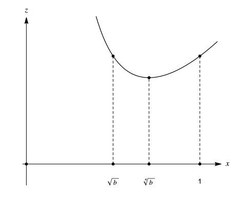
Figure 1. Cauchy-Schlömilch transformation (16).
Looking at Figure 1, we infer that integral (5a) has to be evaluated splitting in two intervals \([\sqrt{b},\sqrt[4]{b}]\) and \([\sqrt[4]{b},1],\) where of course in the first using (8) we have to choose the “-” sign, while in the second integral we have to take the “+” sign. Then using the denesting relation for quadratic surds, solving for \(x\) in (8) we arrive at:
Now, comparing equation (11) and (10), representing the complete elliptic integral of first kind in terms of Gauss \(_2{\rm F}_1\) function, we obtain (4), recalling relation \(c^2+b^2=1.\)
The second result comes from the evaluation of (3) when \(k=3\).
where, to simplify the notation, we put \(n^3=b\) being \(0< n< 1.\) In fact, observing that from (14) follows:
\[
\cos^2\varphi=\frac{x^3-b^2}{c^2}
\]
then, differentiating (14) we find
\[
\frac{-3x^2}{c^2}{\rm d}x=2\sin\varphi\cos\varphi\,{\rm d}\varphi=2\frac{\sqrt{1-x^3}}{c}\frac{\sqrt{x^3-b^2}}{c}{\rm d}\varphi
\]
which shows (15). Legendre then uses again a Cauchy-Schlömilch transformation
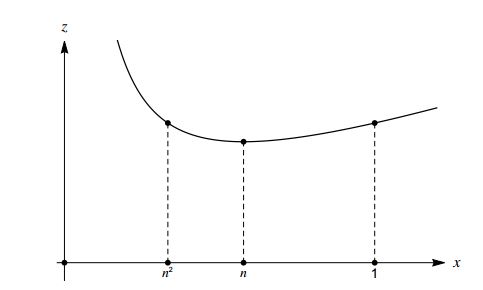
We repeat the same consideration to use correctly the change of variable (16): the lack of monotonicity requires again to split the interval of integration. Looking at Figure 2, we have to split the interval of integration in \([n^2,n]\) and \([n,1]\), recall that \(n< 1.\)
Figure 2. Cauchy-Schlömilch transformation (16)
To work with variable transformation (16) we revisit Legendre’s path, providing a more rigorous approach, in order to manage properly the separation of the domain of integration. First write (16) as:
We now use (20) to get the differential term of the change of variable (16), observe that since \(x\in[n^2,n]\) the (16) transformation is decreasing, see
Figure 2, therefore when \(x\in[n^2,n]\) we have
and solving for \(x\) in (16) always minding that \(x\in[n^2,n]\) we get:
\[
x=\frac{1}{2} \left(z-\sqrt{z^2-4 n^2}\right).
\]
Eventually, after heavy computations helped by computer algebra, we arrive at:
Now factoring we can write:
\[
1+n^6+3 n^2 z-z^3=\left(n^2+1-z\right) \left(\left(z+\frac{n^2+1}{2} \right)^2+
\left(\frac{\sqrt3(1-n^2)}{2}\right)^2\right)
\]
and then we use entry 259.00 page 133 of [15] to provide the left hand side of (26) in terms of complete elliptic integral of first kind:
On the other side, we can evaluate \(R_3(c)\) using the hypergeometric function:
\[
R_3(c)=\frac{\pi}{2}\,_{2}\mathrm{F}_{1}\left( \left.
\begin{array}{c}
\frac12;\frac13 \\[2mm]
1
\end{array}
\right| c^2\right).
\]
Thesis (13) follows representing the complete elliptic integral of first kind in terms of Gauss \(_2{\rm F}_1\) function, replacing \(b\) with \(b^3\) in (27) and (12).
Conclusion
Legendre in his Traité [5] was committed in searching identities among first kind complete elliptic integrals of different moduli, inspired by famous modular transformation:
\begin{equation*}\label{landen}
\mathbf{K}(k)=\frac{1}{1+k}\mathbf{K}\left(\frac{2\sqrt{k}}{1+k}\right).
\end{equation*}
Searching for similar transformations he represented several kind of integrals in terms of complete elliptic integrals of first kind. Our contribution, starting from the elliptic evaluation of integrals \(R_3(c)\) and \(R_4(c)\), see (3), consists of the hypergeometric evaluation of such integrals, which leads to new, for the best of our knowledge, functional relations for the Gauss hypergeometric function, formulae, (4) and (13). A possible new research scenario consists of investigating further hypergeometric relations arising from integrals \(R_k(c)\) when \(k>4.\)
Competing Interests
The author(s) do not have any competing interests in the manuscript.
Acknowledgments
The second author is supported by an Italian RFO research grant.
References
Mingari Scarpello, G. , & Ritelli, D. (2009). The hyperelliptic integrals and \(\pi\). Journal of Number Theory, 129(12), 3094-3108.
Mingari Scarpello, G., & Ritelli, D. (2011). \(\pi\) and the hypergeometric functions of complex argument. Journal of Number Theory, 131, 1887–1900. [Google Scholor]
Mingari Scarpello, G., & Ritelli, D. (2014). Legendre hyperelliptic integrals, \(\pi\) new formulae and Lauricella functions through the elliptic singular moduli. Journal of Number Theory, 135, 334-352.[Google Scholor]
Mingari Scarpello, G., & Ritelli, D. (2014). On computing some special values of multivariate hypergeometric functions. Journal of Mathematical Analysis and Applications, 420(2), 1693-1718.[Google Scholor]
Legendre, A. M. (1825). Traité des fonctions elliptiques et des intégrales eulériennes avec des tables pour en faciliter le calcul numérique, vol. 1. Huzard-Courcier, Paris. [Google Scholor]
Goursat, É. (1881). Sur l’équation différentielle linéaire, qui admet pour intégrale la série hypergéométrique. In Annales scientifiques de l’École Normale Supérieure (Vol. 10, pp. 3-142).[Google Scholor]
Almkvist, G., Van Straten, D., & Zudilin, W. (2011). Generalizations of Clausen’s formula and algebraic transformations of Calabi–Yau differential equations. Proceedings of the Edinburgh Mathematical Society, 54(2), 273-295. [Google Scholor]
Maier, R. (2007). Algebraic hypergeometric transformations of modular origin. Transactions of the American Mathematical Society, 359(8), 3859-3885. [Google Scholor]
Vidūnas, R. (2009). Algebraic transformations of Gauss hypergeometric functions. Funkcialaj Ekvacioj, 52(2), 139-180. [Google Scholor]
Cooper, S., Ge, J., & Ye, D. (2015). Hypergeometric transformation formulas of degrees 3, 7, 11 and 23. Journal of Mathematical Analysis and Applications, 421(2), 1358-1376.[Google Scholor]
Aycock, A. (2013). On proving some of Ramanujan’s formulas for \(\frac {1}{\pi}\) with an elementary method. arXiv preprint arXiv:1309.1140.[Google Scholor]
Amdeberhan, T., Glasser, M. L., Jones, M. C., Moll, V. H., Posey, R., & Varela, D. (2010). The Cauchy-Schlömilch transformation. arXiv preprint arXiv:1004.2445.
Legendre, A. M. (1816). Exercices de calcul intégral sur divers ordres de transcendantes et sur les quadratures (Vol. 3). Courcier. [Google Scholor]
Byrd, P. F., & Friedman, M. D. (1971). Handbook of Elliptic Integrals for Engineers and Scientists 2nd Ed. Springer. [Google Scholor]
Gradshteyn, I. S., & Ryzhik, I. M. (2014). Table of integrals, series, and products. Academic press.
[Google Scholor]