Fractional frequency Laplace transform by inverse difference operator with shift value

1. Introduction

The continuous fractional calculus has been developed by Miller and Ross [1], Oldham and Spanier [2], and Podlubny [3]. Recently discrete delta fractional calculus have been developed by Atici and Eloe [4, 5, 6], Goodrich [7, 8, 9], and Holm [10]. These theories are used in integral transforms in the literature and are applied in astronomy, physics and engineering. The integral transforms like mellin, Laplace and Fourier were applied to obtain the solution of differential equations. These transforms made effectively possible changes a signal in the time domain into a frequency s-domain in the field of Digital Signal Processing(DSP) [11].

The delta Laplace transform was first defined in a very general way by Bohner and Peterson [12]. In 2015, Aleksandar Ivic discussed the discrete Laplace transforms in the view of fast decay factor \(e^{-sx}\) and obtained the Laplace transform of \(P(x)\) as \(\int\limits_{0}^{\infty}P(x)e^{-sx}dx=\pi s^{-2}\sum\limits_{n=1}^{\infty}r(n)e^{-\pi^2/n}\). In practice, many applications of Laplace Transform (LT), \(L[f(x)]=\int\limits_{0}^{\infty}f(x)e^{-sx}dx\), and the forward Discrete Laplace Transform (DLT), \(L[f(n)]=\sum\limits_{n=0}^{\infty}f(n)e^{-sn}\), are discussed and mentioned by several authors in the citations [13, 14, 15, 16].

In the existing Laplace transform the shifting value of time domains are one. In 2016, G. Britto Antony Xavier etc., [17] have defined Laplace transform with shift value \(\ell\) using generalized difference operator and obtain the outcomes of polynomial and trigonometric functions etc. In this fractional Laplace transform with shift value \(\nu\) taken from 0 to 1.

In this paper, we continue the work derived in [17] by defining fractional frequency Laplace transform with fractional factor \(e^{-s^{1/\nu}t}\). We presented convolution product and several properties of the fractional transforms for the functions like polynomial factorial and trigonometric functions.

2. Preliminaries

In this section, we present basic theory of the \(\ell-\)difference operator \(\Delta_h\). The polynomial factorial is defined \(t_{h}^{(m)}=t(t-h)(t-2h)\cdots (t-(m-1)h)\), \(h>0\) for non-negative integer \(m\) and using Stirling numbers\newpage \noindent of first kind \(s_{r}^{m}\) and second kind \(S_{r}^{m}\), the relation between polynomial and polynomial factorials are given by,

Definition 1. Let \(u(t),\ t\in[0,\infty)\), be a real or complex valued function and \(h>0\) be a fixed shift value. Then, the \(h-\)difference operator \(\Delta_{h}\) on \(u(t)\) is defined as

and its infinite \(h-\) difference sum is defined by

Definition 2. Let \(u(t)\) and \(v(t)\) are the two real valued functions defined on \((-\infty,\infty)\) and if \(\Delta_h v(t)=u(t),\) then the finite inverse principle law is given by

Applying the Definition 1, we get the modified identities as follows:

Lemma 3. [18] Let \(h>0\) and \(u(t)\), \(w(t)\) are real valued bounded functions. Then

Lemma 4. Let \(t\in (-\infty, \infty),\,\,h>0\) and \(\nu>0\), then we have

Proof. The proof follows by taking \(u(t)=e^{-s^{1/\nu}t}\) in Definition 1 and applying \(\Delta_h^{-1}\).

Corollary 5. Let \(t\in (-\infty, \infty),\,\,h>0\) and \(\nu>0\), then we have

Proof. The proof follows by equating (7) and the finite inverse principle law given in (4).

Example 1.For the particular values \(\nu=0.5,\,s=0.1,\,t=3\) and \(h=2\), (8) is verified by MATLAB. The coding is given by \((2.*exp(-(0.1).\wedge(1./0.5).*3))./(exp(-(0.1).\wedge(1./0.5).*2)-1)-(2.*exp(-(0.1).\wedge(1./0.5).*1))./(exp(-(0.1).\wedge(1./0.5).*2)-1)=2.*symsum(exp(-(0.1).\wedge(1./0.5).*(3-2.*r)),r,1,1)\).

Theorem 6. Let \(t\in (-\infty, \infty)\), \(h>0\) be shift value and \(2(\cosh s^{{1}/{\nu}}h-\cos ph)\neq0\). Then we have

Proof. Taking \(\Delta_{h}^{-1}\) on \(u(t)=e^{-s^{{1}/{\nu}}t}\cos pt\), we get: $$\Delta_{h}^{-1}(e^{-s^{{1}/{\nu}}t}\cos pt)=\text{Re\ part\ } \Delta_{h}^{-1}(e^{-s^{{1}/{\nu}}t}e^{ipt})=\text{Re\ part\ } \Delta_{h}^{-1}(e^{(-s^{{1}/{\nu}}+ip)t} ),$$ Now (9) follows by applying Lemma 4 and taking conjugate. Similarly the proof of (10) holds.

3. Fractional Frequency Laplace Transform and its Properties

In this section, we define and obtain the properties of FGLT and present the transforms of certain functions like trigonometric, hyperbolic and polynomials etc.

Definition 7. Let \(u(t)\) be the real valued function, \(h>0\) and \(\nu\in {R^+}\). If \(\lim\limits_{t\rightarrow \infty}\Delta_h^{-1}u(t)e^{-s^{{1}/{\nu}}t}=0\), then the Fractional Frequency Laplace Transform(FFLT) is defined as

Proposition 8. If \(L_{h,\nu}(u(t))=\bar{u}_{h,\nu}(s)\) and \(L_{h,\nu}(v(t))=\bar{v}_{h,\nu}(s)\), then

Proof. From (11), we have \(L_{h,\nu}(u(at))=\Delta_{h}^{-1}u(at)e^{-s^{1/\nu}t}\big |_{t=0}^{\ \infty}\). Now the proof follows by substituting \(at\) by \(k\).

Proposition 9. \label{L555} If \(L_{h,\nu}(u(t))=\bar{u}_{h,\nu}(s)\), then \(L_{h,\nu}(e^{-at}u(t))=\bar{u}_{h,\nu}(s+a).\)

Proof. The proof follows by taking \(u(t)=e^{-at}u(t)\) in (11).

Theorem 10. If \(\cosh s^{{1}/{\nu}}h-\cos ph\neq 0\), then we have

When \(h\rightarrow 0\) and \(\nu=1\), we get \(L(\sin pt)=\dfrac{p}{s^2+p^2}\) and \(L(\cos pt)=\dfrac{s}{s^2+p^2}.\)

Proof. The proof of (13) follows from (9), (10) and (11).

Theorem 11. If \(\cosh s^{1/\nu}h-\cos(n-2r)ph\neq 0\) for \(r=0,1,2,\cdots,n\), then

Proof. From \(\sin^{n}pt=\dfrac{1}{2^{n-1}(-1)^{\frac{n-1}{2}}}\sum\limits_{r=0}^{[n/2]}(-1)^r\binom{n}{r}\sin(n-2r)pt\) and (13), we get the proof of (14). Similarly we can obtain the proof of (15), (16) and (17).

Corollary 12. Let \(t\in [0,\infty)\), \(s,h,nu>0\), then we have

Proof. The proof follows by taking \(n=5\) in (14) and then equating that with (11).

Example 2.For the particular values \(\nu=0.6,\,s=3,\,p=2\) and \(h=3\), (18) is verified by MATLAB. The coding is given by \(3.*symsum((sin(2.*3.*r)).\wedge 5.*exp(-3.\wedge(1./0.6).*3.*r),r,0,inf)=(3.*sin(5.*2.*3))./(32.*(cosh((3).\wedge(1./0.6).*3)-cos(5.*2.*3)))-(5.*3.*sin(3.*2.*3))./(32.*(cosh((3).\wedge(1./0.6).*3)-cos(3.*2.*3)))+(10.*3.*sin(2.*3))./(32.*(cosh((3).\wedge(1./0.6).*3)-cos(2.*3))) \).

Theorem 13. If \(e^{-(s^{1/\nu}\pm p)h}\neq 1\) and \(s>0\), then

When \(h\rightarrow 0\) and \(\nu=1\), we get \(L(\sinh pt)=\dfrac{p}{s^2-p^2}\) and \(L(\cosh pt)=\dfrac{s}{s^2-p^2}.\)

Proof. From (11), we have \(L_{h,\nu}(\sinh pt)=(1/2)\Delta_{h}^{-1}e^{-s^{1/\nu}t}(e^{pt}-e^{-pt})\). Which completes the proof of (19). Similarly we can obtain \(L_{h,\nu}(\cosh pt)\).

Theorem 14. If we denote \(H_r=e^{-(s^{1/\nu}+(n-2r)a)h}-1\), \(H_{-r}=e^{-(s^{1/\nu}-(n-2r)a)h}-1\), then

Proof. From \(\sin h^{n}pt=\dfrac{1}{2^{n-1}}\sum\limits_{r=0}^{[n/2]}(-1)^r\binom{n}{r}\sin h(n-2r)pt\) and (13), we get the proof of (20). Similarly, we can obtain the proof of (21), (22) and (23).

Theorem 15. Let \(t\in (0,\ \infty)\), \(h>0\) and \(s>0\), then \(L_{h,\nu}(t_{h}^{(\mu)})=\dfrac{h^{\mu+1}\mu!e^{s^{1/\nu}h}}{(e^{s^{1/\nu}h}-1)^{\mu+1}}\).

Proof. Taking \(u(t)=t_{h}^{(1)}\) in (11), we have \(L_{h,\nu}(t_{h}^{(1)})=h\Delta_{h}^{-1}e^{-s^{1/\nu}t}t_{h}^{(1)}\big |_{t=0}^{\ \infty}\). Now taking \(u(t)=t_{h}^{(1)}\), \(w(t)=e^{-s^{1/\nu}t}\) in (6) and applying (5), we get

Now taking \(u(t)=t_{h}^{(2)}\) in (11) and applying (6), and (5), we get \(L_{h,\nu}(t_{h}^{(2)})=\dfrac{h^32!e^{s^{1/\nu}h}}{(e^{s^{1/\nu}h}-1)^3}.\) Repeating this process \(n\) times, we get the proof of Theorem 15.

Corollary 16.\label{L17} Let \(t\in (0,\ \infty)\), \(h>0\) and \(s>0\), then \(L_{h,\nu}(t^n)=\sum\limits_{r=0}^{n}\dfrac{S_{r}^nh^{n+1}n!e^{s^{1/\nu}h}}{(e^{s^{1/\nu}h}-1)^{n+1}}\).

Proof. The proof follows from \((ii)\) of (1), \((ii)\) of (5) and Theorem (15).

Example 3.Taking \(n=2\) in Theorem 15, we obtain

which verified for the values \(h=2,s=3\) and \(\nu=0.7\) by MATLAB coding given below: \(2.*symsum((r.*2.*(r-1).*2).*exp(-3.\wedge(1./0.7).*r.*2),r,0,inf)=(16.*exp(3.\wedge(1./0.7).*2))./((exp(3.\wedge(1./0.7).*2)-1).\wedge3).\)

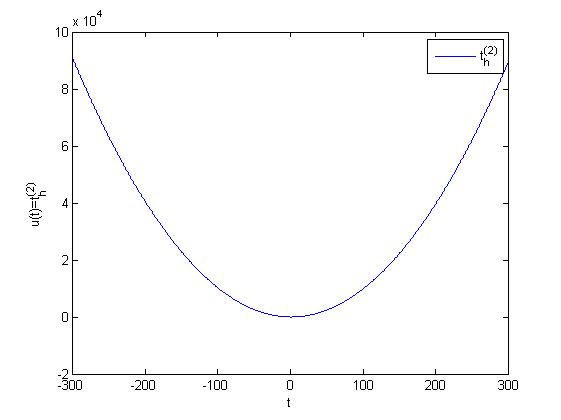
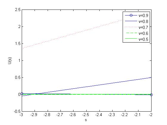
Figure 1 is the input function(signal) as polynomial factorial for the time factor \(t\) and Figure 2 is the fractional generalized Laplace transform in the frequency domain \(s\) and also here in the frequency domain the fraction \(\nu\) varies as \(0.9,0.8,0.7,0.6,0.5\) which are generated by MATLAB.

4. Convolution Product and Fractional Laplace Transforms

In this section, we defined convolution product and its properties with Fractional Laplace transforms. The following definitions are motivated by [19] using difference operator.

Definition 17. Let \(u(t)\) be the real valued function, then the incomplete generalized Laplace transform is defined by

Definition 18. Let \(u(t)\) and \(v(t)\) are the two real valued functions, then the convolution product is defined by

The following lemma shows that the relation between convolution product and Fractional Laplace transform.

Lemma 19. Let \(\mu\in R^+,\) \(u(t)\) and \(v(t)\) are the real valued functions, then

\item \(u\circ e^{-\mu^{1/\nu}}=L_{h,\nu}[u]\cdot e^{-\mu^{1/\nu}}\), \item \(L_{h,\nu}[u\circ v]=L_{h,\nu}[L_h(u(t_1),\xi)]\).

Proof. (1) From (27), we get \((u\circ e^{-\mu^{1/\nu}})(t)=\Delta_h^{-1}u(\xi-t)e^{-\mu^{1/\nu}t}\big|_{\xi=t}^\infty\). Taking \(t_1=\xi-t\), which gives \((u\circ e^{-\mu^{1/\nu}})(t)=\Delta_h^{-1}u(t_1)e^{-\mu^{1/\nu}(t_1+t)}\big|_{t_1=0}^\infty\). Then, \((u\circ e^{-\mu^{1/\nu}})(t)=e^{-\mu^{1/\nu}(t)}\Delta_h^{-1}u(t_1)e^{-\mu^{1/\nu}(t_1)}\big|_{t_1=0}^\infty\), which completes the proof of (1).\\ (2) Now \(L_{h,\nu}[u\circ v](t)=\Delta_h^{-1}(u\circ v)(t)e^{-\mu^{1/\nu}(t)}\Big|_{t=0}^\infty=\Delta_h^{-1}\left[\Delta_h^{-1}u(\xi-t)v(\xi)\big|_{\xi=t}^\infty\right]e^{-\mu^{1/\nu}(t)}\Big|_{t=0}^\infty\). Now applying Fubini's Theorem, we get

Then the proof of (2) follows by applying (26).

The following example illustrate the verification of convolution product.

Example 4. Consider the following functions $$u(t)=\begin{cases} e^{-s^{1/\nu}t} ,\quad\ t\in(0,\infty)\\ \ \ 0, \qquad\quad \text{otherwise}\end{cases}\quad v(t)=\begin{cases} t ,\quad\ t\in(0,\infty)\\ 0, \quad \text{otherwise}\end{cases}$$ Now, from (27), we get \((u\circ v)(t) = \Delta_h^{-1}e^{-s^{1/\nu}(\xi-t)}\xi\Big|_{\xi=0}^\infty.\) Then using (24), which gives \((u\circ v)(t)=\dfrac{h^2e^{-s^{1/\nu}(h-t)}}{(e^{-s^{1/\nu}h}-1)^2}\). By (3), we get the relation as follows \begin{equation*} (u\circ v)(t)=h\sum\limits_{r=0}^{\infty}(rh)e^{-s^{1/\nu}(rh-t)}=\dfrac{h^2e^{-s^{1/\nu}(h-t)}}{(e^{-s^{1/\nu}h}-1)^2} \end{equation*} which verified for the values \(t=4,h=3,s=2\) and \(\nu=0.3\) by MATLAB coding given below: \(3.*symsum(exp(-2.\wedge(1./0.3).*((r.*3)-4)).*r.*3,r,0,inf)=9.*exp(-2.\wedge(1./0.3).*(-1))./((exp(-2.\wedge(1./0.3).*3)-1).^2).\)

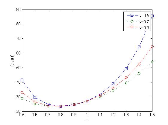
Figure 3 explains the input time(t) function \(u(t)\) and \(v(t)\) and Figure 4 tells that the convolution product of the functions in the frequency(s) domain as varying \(\nu\) as \(0.5,0.6,0.7\) which are generated by MATLAB.

5. Conclusion

The fractional generalized Laplace transform is successfully defined and properties were presented. We derived formulaes and obtained its transform for certain functions like polynomial factorial, trigonometric functions, etc. When \(\nu=1\) and \(h\rightarrow 0\), we get classical Laplace transform. The convolution product defined and the relation between Laplace transform and convolution product were presented. We conclude this investigations and findings are verified and analyzed the outcomes in the time(t) and frequency(s) domains with graphs.

Author Contributions

All authors contributed equally to the writing of this paper. All authors read and approved the final manuscript.

Competing Interests

The author(s) do not have any competing interests in the manuscript.

References

Miller, K. S., & Ross, B. (1993). An introduction to the fractional calculus and fractional differential equations. John Wiley & Sons, Inc., New York. [Google Scholor]
Oldham, K., & Spanier, J. (2002). The fractional calculus theory and applications of differentiation and integration to arbitrary order. Dover Publications, Inc., Mineola, New York.[Google Scholor]
Podlubny, I. (1998). Fractional differential equations: an introduction to fractional derivatives, fractional differential equations, to methods of their solution and some of their applications (Vol. 198). Elsevier. [Google Scholor]
Atici, F. M., & Eloe, P. W. (2011). Two-point boundary value problems for finite fractional difference equations. Journal of Difference Equations and Applications, 17(04), 445-456. [Google Scholor]
Atici, F. M., & Eloe, P. W. (2007). Fractional q-calculus on a time scale. Journal of Nonlinear Mathematical Physics, 14(3), 341-352.[Google Scholor]
Atici, F. M., & Eloe, P. W. (2007). A transform method in discrete fractional calculus. International Journal of Difference Equations, 2(2), 165-176. [Google Scholor]
Goodrich, C. S. (2010). Solutions to a discrete right-focal fractional boundary value problem. International Journal of Difference Equations, 5(2), 195-216.[Google Scholor]
Goodrich, C. S. (2010). Continuity of solutions to discrete fractional initial value problems. Computers & Mathematics with Applications, 59(11), 3489-3499. [Google Scholor]
Goodrich, C. S. (2011). Some new existence results for fractional difference equations. International Journal of Dynamical Systems and Differential Equations, 3(1-2), 145-162.[Google Scholor]
Holm, M. (2011). Sum and difference compositions in discrete fractional calculus. Cubo (Temuco), 13(3), 153-184.[Google Scholor]
Smith, S. W. (1997). The scientist and engineer’s guide to digital signal processing(Second Edition). California Technical Publishing San Diego, California.[Google Scholor]
Bohner, M., & Peterson, A. (2012). Dynamic equations on time scales: An introduction with applications. Springer Science & Business Media. [Google Scholor]
Ivic, A. (2015). Some applications of Laplace transforms in analytic number theory. Novi Sad Journal of Mathematics, 45(1), 31-44. [Google Scholor]
Ivic, A. (2000). The Laplace transform of the fourth moment of the zeta-function. Publikacije Elektrotehnickog fakulteta. Serija Matematika, 41-48. [Google Scholor]
Sedletskii, A. M. (2014). Fourier transforms and approximations. CRC press. [Google Scholor]
Jutila, M. (2001). The Mellin transform of the square of Riemann’s zeta-function. Periodica Mathematica Hungarica, 42(1-2), 179-190.[Google Scholor]
G. Britto Antony Xavier, B. Govindan, S. John Borg and M. Meganathan, Generalized Laplace Transform arrived from an Inverse Difference Operator, Global Journal of Pure and Applied Mathematics, 12(3) (2016),661-666. [Google Scholor]
Britanak, V., & Rao, K. R. (1999). The fast generalized discrete Fourier transforms: A unified approach to the discrete sinusoidal transforms computation. Signal Processing, 79(2), 135-150.[Google Scholor]
Medina, G. D., Ojeda, N. R., Pereira, J. H., & Romero, L. G. (2017). Fractional Laplace Transform and Fractional Calculus. International Mathematical Forum, 12(20), 991-1000.[Google Scholor]