Cervical cancer is a global threat with over half a million cases worldwide and over 200000 deaths annually. Sexual minority women are at risk for infection with human papillomavirus (HPV); the virus which causes cervical cancer, yet little is known about the prevalence of HPV infection. In this paper, the dynamics of HPV infection in the presence of vaccination among women which progresses to cervical cancer is investigated. The disease-free equilibrium state of the model is determined. Using the next generation method, the cancer reproduction number, \(R_0\), is computed in terms of the model parameters and used as a threshold value. The reproduction number is examined analytically for its sensitivity to the vaccination parameter having shown that it is locally and globally asymptotically stable for \(R_0<1\) and unstable for \(R_0>1\) at the disease free state. The centre manifold theorem is used to determine the stability of the endemic equilibrium and shown to exhibit a backward bifurcation phenomenon implying that cervical cancer due to HPV infection may persist in the population even if \(R_0<1\). Finally, numerical simulations are carried out to obtain analytical results. As prevalence estimates vary between sexual orientation dimensions, these findings help inform targeted HPV and cervical cancer prevention efforts.
The human body is composed of cells which reproduce and generate new cells. However the abnormal growth of these cells leads to cancer.
There are different types of cancers, and the location where a cancer begins defines its name even though it can spread to different parts of the body [1]. Human Papillomavirus is now a well established cause of cervical cancer and is the most common related viral infection of the reproductive system. Persistent HPV infection leads to precancerous cells in the cervix which later become malignant.
Human Papillomavirus is transferred from one person to the other through skin contact but not through blood [2]. Over \(100\) different HPV strains have been discovered and classified among which \(16, 18, 31\) and \(45\) are referred to as high risk [3].
HPV strain \(16\) and \(18\) have been accounted to cause \(70\%\) of cervical cancers [4]. In general, there are no signs that show that one has genital HPV apart from the genital warts caused by the types \(6\) and \(11\). However, most HPV infections go away naturally [5].
Cervical cancer is the chief cause of death among cancer related deaths in women especially in developing countries [6,7 ]. The world population is at risk of developing cervical cancer with statistics showing that girls and women aged \(15\) years and older having HPV is about 2.8 million [8].
Over half a million women across the world are diagnosed with cervical cancer with about \(265,672\) dying from the disease annually [8].
Approximately \(3000\) Ghanaian women are diagnosed with cervical cancer each year with about \(2000\) of the cases leading to death. In Uganda and Nigeria, about \(3915\) and \(14089\) women are recorded of having cervical cancer and \(2275\) and \(8240\) out of the recorded cases die from the disease respectively [9]. Each year over \(500000\) cases are diagnosed worldwide with \(200000\) deaths relating to this disease [1].
Many researchers have used mathematical models to explain the dynamics of HPV infection leading to cervical cancer and the intervention strategies [2, 7, 10, 11, 12]. Pongsumpun analysed a mathematical model of cervical cancer due to HPV [1]. Pongsumpun observed that, for a given period of time when the number of women infected with HPV is higher, the time of convergence for one to be infected becomes shorter.
Although a model incorporating screening was developed by [13] in the effort of reducing HPV infection incidence in the population, vaccination plays a major role in reducing HPV infection by protecting both vaccinated and unvaccinated individuals. Motivated by this assertion of reduction in HPV infections as a result of vaccination; a mathematical model of cervical cancer due to HPV infection incorporating vaccination is constructed. The rest of the paper is organized as follows: Section 2 provides the model formulation. Section 3 presents the analysis of the model. Numerical simulations are carried out in Section 4 and finally, the discussion is presented in Section 5.
2. Basic Model Formulation
In this section, the formulation of the model for the transmission of HPV in the presence of vaccination which classifies the population at any time \(t\) into compartments depending on the infection status of an individual is made. The total population at time \(t\) is denoted by \(N(t)\) and it is divided among five disjoint independent compartments. These are: the compartment denoted by \(S\) which contains the susceptible individuals. \(I(t)\) refers to the number of infectious individuals in the population, \(V(t)\) refers to the number of individuals who are vaccinated, \(C(t)\) is the number of individuals with cervical cancer, and \(R\) refers to the compartment of the recovered individuals. We assume that individuals are recruited into the susceptible compartment at a constant rate \(\pi\). A proportion \(\theta\) of these individuals in the susceptible population are vaccinated. The vaccine offers some protection against the infection. However, the susceptible individuals can be infected by HPV at a rate \(\lambda\) when they come into effective contact of an infectious individual. The parameter \(\beta\), is the effective contact rate. The vaccine is assumed to wane and vaccinated individuals can become susceptible again. The vaccine wanes at a rate \(\omega\). However, a positive modification of the lesbian and bisexual women behaviour by a rate \(\eta\) influences the contact rate of \(C(t)\) and brings about a reduction in the infectivity potential of transmission rate of HPV in the population. The force of infection is given by \(\lambda = \dfrac{\beta(I + \eta C)}{N}\). Furthermore, we assume that the individuals who receive vaccination may be infected at a reduced rate \((1 – \epsilon)\lambda\), where \(\epsilon \in (0,1)\) measures the efficacy of the vaccine. If \(\epsilon = 0\), then the vaccine is useless and if \(\epsilon = 1\), then the vaccine is \(100\%\) effective in preventing HPV infection. Moreover, the infected individuals progress to develop cervical cancer at a rate \(\sigma\) while those who do not develop cancer recover at a rate \(\gamma_1\). Individuals with cervical cancer recover at a rate \(\rho\). The parameter \(\gamma_2\) denotes the rate at which those who progress to develop cervical cancer recover from HPV and cancer. Individuals in each compartment die naturally at a rate \(\mu\), while mortality as a result of cervical cancer is given by \(\alpha\). The general process of this model is shown in Figure 1.
Figure 1. Flow diagram for HPV infection with vaccination.
From the assumptions made and the flow diagram, we obtain the following system of non linear ordinary differential equations;
\begin{equation}\label{eq. 1}
\left.\begin{aligned}
\frac{dS}{dt} & = \pi + \omega V – (\lambda + \theta + \mu)S, \\[5pt]
\frac{dV}{dt} & = \theta S – (1 – \epsilon)\lambda V – (\mu + \omega)V, \\[5pt]
\frac{dI}{dt} & = \lambda S + (1 – \epsilon)\lambda V + \rho C – (\sigma + \gamma_1 + \mu)I, \\[5pt]
\frac{dC}{dt} & = \sigma I – (\rho + \gamma_2 + \mu + \alpha)C, \\[5pt]
\frac{dR}{dt} & = \gamma_1 I + \gamma_2 C – \mu R.
\end{aligned}
\right\}
\end{equation}
(1)
The initial conditions of our system are: \(S(0)>0\) and \(V(0)\), \(I(0)\), \(C(0)\), \(R(0)\) \(\geq 0\). Since the model sub-divides the total population into five different compartments, it implies that $$N(t) = S(t) + V(t) + I(t) + C(t) + R(t).$$ Hence, the rate at which the total population is changing over a period of time is thus
\begin{align}\label{a}
\frac{dN}{dt} &= \pi – \mu N – \alpha C \leq \pi -\mu N.
\end{align}
(2)
3. Model Analysis
3.1. Positivity and boundedness of solutions
For the model system (1) to be epidemiologically meaningful, we prove that all state variables are non-negative. Since it is irrational to have a negative population density and system (1) describes the dynamics of the human population; we show that all state variables are positive and the solutions of system (1) with positive initial conditions will remain positive for fall \(t > 0\). The following lemma is applied.
Lemma 1.
Given that the initial solutions and parameters of system (1) are positive, the solutions \(S(t)\), \(V(t)\), \(I(t)\), \(C(t)\) and \(R(t)\) are non-negative for all \(t > 0\).
Proof.
We define $$\hat{t} = \sup\{t>0: S(t)>0\quad \text{and}\quad V(t), I(t), C(t), R(t) \geq 0 \}. $$
This implies that
$$ S(t)>0,\quad \text{and}\quad V(t), I(t), C(t), R(t) \geq 0\quad \forall\quad t \in [0, \hat{t}).$$
Considering the first equation in system (1) we have:
$$
\frac{dS}{dt} = \pi + \omega V – (\lambda + \theta + \mu)S.\qquad\quad\quad
$$
Since \(\pi\) and \(\omega\) are positive, we have
$$
\frac{dS}{dt} \geq -(\lambda + \theta + \mu)S(t), \quad \forall \quad t \in [0,\hat{t}).
$$
Separating variables, we obtain
\begin{align*}
\frac{d S}{S} & \geq – (\lambda + \theta + \mu)dt. \qquad \qquad \qquad \quad
\end{align*}
We integrate both sides between \(0\) and \(\hat{t}\) to have,
\begin{align*}
\int_{0}^{\hat{t}} \frac{dS}{S} & \geq \int_{0}^{\hat{t}} – (\lambda + \theta + \mu) dt, \qquad \qquad\quad \quad
%\bigg[\ln (S)\bigg]_{0}^{\hat{t}} & \geq – \bigg(\theta \hat{t} + \mu \hat{t} + \int_{0}^{\hat{t}} \lambda dt\bigg), \\[5pt]
%\ln S(\hat{t}) – \ln S(0) &\geq – \bigg(\theta \hat{t} + \mu \hat{t} + \int_{0}^{\hat{t}} \lambda dt\bigg). \qquad
\end{align*}so that
\begin{align*}
%\exp (\ln S(\hat{t}) – \ln S(0)) & \geq \exp\bigg[ – \bigg(\theta \hat{t} + \mu \hat{t} + %\int_{0}^{\hat{t}} \lambda dt \bigg)\bigg],\qquad\qquad\quad \quad \quad \\[5pt]
S(\hat{t}) & \geq S(0) \exp \bigg[ – \bigg(\theta \hat{t} + \mu \hat{t} + \int_{0}^{\hat{t}} \lambda dt \bigg)\bigg]>0.
\end{align*}
From the second equation of system (1) we obtain,
\begin{align*}
\quad \qquad \quad\frac{dV}{dt} & = \theta S – (\omega + (1- \epsilon)\lambda + \mu)V, \quad\\[5pt]
\implies \frac{dV}{dt}& \geq -(\omega + (1 – \epsilon)\lambda + \mu)V(t),\quad \forall t \in [0,\hat{t}).
\end{align*}
Through integration we have
\begin{align*}
V(\hat{t}) & \geq V(0) \exp\bigg[ -\bigg(\omega \hat{t} + \mu \hat{t} + \int_{0}^{\hat{t}} (1 – \epsilon)\lambda dt \bigg)\bigg] \geq 0.
\end{align*}
Similarly for the third equation of system (1) we get,
\begin{align*}
I(\hat{t}) & \geq I(0) \exp \bigg[- \hat{t}(\sigma + \gamma_1 +\mu)\bigg] \geq 0.
\end{align*}
For the fourth equation of system (1) we also have,
\begin{align*}
C(\hat{t}) & \geq C(0) \exp [-\hat{t} (\rho + \gamma_2 + \mu + \alpha)] \geq 0.
\end{align*}
Lastly, from the fifth equation of system (1) we obtain,
\begin{align*}
R(\hat{t}) & \geq R(0) \exp [-\mu \hat{t}] \geq 0.
\end{align*}
In conclusion, \(S(t)>0\) and \(V(t)\), \(I(t)\), \(C(t)\), \(R(t)\) \(\geq 0\) for all \(t > 0\) given that: $$S(0)>0 \quad \text{and}\quad V(0), I(0), C(0), R(0) \geq 0.$$
The biologically feasible region \(\mathcal{D} = \{(S, V, I, C, R) \in \mathbb{R}_{+}^{5}: N \leq \frac{\pi}{\mu}\}\) is defined such that summing all the equations of system (1) gives (2). Applying the integration factor method which is used for solving linear first-order differential equations on Equation (2) we have,
\begin{align*}
N(t) & = \frac{\pi}{\mu} + \bigg(N(0) – \frac{\pi}{\mu} \bigg)e^{-\mu t}.
\end{align*}
Hence, as \(t \longrightarrow \infty\), \( N(t) \longrightarrow \dfrac{\pi}{\mu}\). Therefore every solution \(N(t)\) of equation (2) satisfies the condition below:
\begin{align*}
0 \leq N(t) \leq N(0)e^{-\mu t} + \dfrac{\pi}{\mu}(1 – e^{-\mu t}),
\end{align*}
where \(N(0)\) is the sum of all the initial conditions of the variables of our model. If \(N(0)\leq \dfrac{\pi}{\mu}\), then the total population at time \(t\) is bounded above by \(\dfrac{\pi}{\mu}\). Therefore, for any solution \(\{S(t)>0, V(t), I(t), C(t), R(t) \geq 0\}\) at \(t > 0\) of system (1) that begins in \(\mathbb{R}_{+}^{5}\), it either remains in or approaches \(\mathcal{D}\) asymptotically. Hence, the region \(\mathcal{D}\) is positively invariant and attracting with respect to system (1).
3.2. Disease-free equilibrium \(E_0\)
At the disease free equilibrium, there is no disease in the system. As a result, there will be no transmission of the disease for an uninfected lesbian and bisexual women to be infected. Also, the absence of transmission of the disease means there will be no recovery. However, vaccination is impose on the susceptible individuals. Thus, the disease-free equilibrium is given by
It can be defined in this context as the expected number of secondary cases, produced by one infectious individual in a totally susceptible or disease free population [14]. It is obtained as
The basic reproduction number is observed to be the sum of two terms \((R_{HPV}+ R_C)\) corresponding to what each of the infected compartments (HPV infection and cancer) are contributing to the epidemic. When \(\beta = 0\); \(R_0 = 0\); no HPV or cancer in the reproduction. When \(\sigma=0\), i.e. when no one progresses to cervical cancer, we only have the reproduction of HPV infection (i.e. \(R_{HPV}\)). Thus, we cannot have cervical cancer without HPV infection so the reproduction number for cervical cancer cannot stand alone.
3.4. Stability analysis of disease-free equilibrium
The stability analysis of the disease-free equilibrium point, \(E_0\), will be investigated in this section.
Theorem 2.
The disease-free equilibrium, \(E_0\), is locally asymptotically stable when \(R_0 < 1\) and unstable otherwise.
Proof.
The proof of the theorem is investigated by the linearization method. The Jacobian matrix associated with the model system (1) at the disease-free equilibrium is given by:
\[
J(E_0) =\left( {
\begin{array}{ccccc}
-(\theta + \mu) \quad & \omega \quad & -\dfrac{\beta(\omega + \mu)}{(\theta + \omega + \mu)} \quad & -\dfrac{\beta \eta (\omega + \mu)}{(\theta + \omega + \mu)} \quad & 0\\
\theta \quad & -(\omega + \mu) \quad & \dfrac{\beta(\theta – \epsilon\theta )}{(\theta + \omega + \mu)} \quad & \dfrac{\beta \eta (\theta – \epsilon \theta)}{(\theta + \omega + \mu)} \quad & 0 \\
0 \quad & 0 \quad & \dfrac{\beta(\omega + \mu + \theta (1-\epsilon))}{(\theta + \omega + \mu)}-(\sigma +\gamma_1 +\mu) \quad & \dfrac{\beta \eta (\omega + \mu + \theta (1-\epsilon))}{(\theta + \omega + \mu)}+ \rho \quad & 0 \\
0 \quad & 0 \quad & \sigma \quad & -(\rho + \gamma_2 + \mu + \alpha) \quad & 0 \\
0 \quad & 0 \quad & \gamma_1 \quad & \gamma_2 \quad & -\mu
\end{array}
}
\right).
\]
Expanding the characteristic equation \(|J(E_0) – \lambda I| = 0\) by the last column, we obtain the eigenvalue of \(J(E_0): \lambda_1 = -\mu\). The other four eigenvalues are the eigenvalues of the \(4 \times 4\) matrix given by:
\[
J_1(E_0) =\left( {
\begin{array}{cccc}
-(\theta + \mu) \quad & \omega \quad & -\dfrac{\beta(\omega + \mu)}{(\theta + \omega + \mu)} \quad & -\dfrac{\beta \eta (\omega + \mu)}{(\theta + \omega + \mu)}\\[5pt]
\theta \quad & -(\omega + \mu) \quad & \dfrac{\beta(\theta – \epsilon\theta )}{(\theta + \omega + \mu)} \quad & \dfrac{\beta \eta (\theta – \epsilon \theta)}{(\theta + \omega + \mu)} \\[5pt]
0 \quad & 0 \quad & \dfrac{\beta(\omega + \mu + \theta (1-\epsilon))}{(\theta + \omega + \mu)}-(\sigma +\gamma_1 +\mu) \quad & \dfrac{\beta \eta (\omega + \mu + \theta (1-\epsilon))}{(\theta + \omega + \mu)}+\rho \\[5pt]
0 \quad & 0 \quad & \sigma \quad & -(\rho + \gamma_2 + \mu+\alpha)
\end{array}
}
\right).
\]
\begin{multline*}
J_1(E_0) = \begin{pmatrix}
A & B \\[20pt]
0 & C
\end{pmatrix},\quad \text{where}\quad A = \begin{pmatrix}
-(\mu+\theta) & \omega \\[20pt]
\theta & -(\mu + \omega)
\end{pmatrix},
\qquad
B = \begin{pmatrix}
-\frac{\beta(\omega + \mu)}{\theta + \omega + \mu} & -\frac{\beta \eta (\omega + \mu)}{(\theta + \omega + \mu)}\\[20pt]
\frac{\beta (\theta – \epsilon \theta)}{(\theta + \omega + \mu)} & \frac{\beta \eta (\theta – \epsilon\theta )}{(\theta + \omega + \mu)}
\end{pmatrix}\\\qquad \qquad \qquad
\end{multline*}
and
\begin{align*}
\qquad C = \begin{pmatrix}
\dfrac{\beta(\omega + \mu + \theta (1-\epsilon))}{(\theta + \omega + \mu)}-(\sigma + \gamma_1 + \mu) & \dfrac{\beta \eta (\omega + \mu + \theta(1-\epsilon))}{(\theta + \omega + \mu)} + \rho \\[20pt]
\sigma & – (\rho + \gamma_2 + \mu + \alpha)
\end{pmatrix}.
\end{align*}
The eigenvalues of \(J_1(E_0)\) are the eigenvalues of \(A\) and \(C\). The characteristic equation of \(A\) and \(C\) is given by
where
\begin{align*}
D = \bigg[(\sigma +\gamma_1 + \mu)(\rho + \gamma_2 + \mu + \alpha)-\dfrac{\beta (\omega + \mu + \theta(1-\epsilon))(\rho + \gamma_2 + \mu + \alpha)}{(\theta + \omega + \mu)} – \dfrac{\beta \eta \sigma (\omega + \mu + \theta (1-\epsilon))}{(\theta + \omega + \mu)} – \sigma \rho\bigg]. \quad
\end{align*}
From C\(= \lambda^2 + \lambda_1 A_{11} + A_{12}\), we have;
\begin{align*}
A_{11} &= (\sigma + \gamma_1 + \mu)\bigg[1 – \bigg(\frac{\beta(\omega + \mu + \theta (1-\epsilon))}{(\sigma + \gamma_1 + \mu)(\theta + \omega + \mu)} \bigg) \bigg] + (\rho + \gamma_2 + \mu +\alpha),\\
A_{12} & =(\sigma +\gamma_1 + \mu)(\rho + \gamma_2 + \mu +\alpha)-\dfrac{\beta (\omega + \mu + \theta(1-\epsilon))(\rho + \gamma_2 + \mu+\alpha)}{(\theta + \omega + \mu)} – \dfrac{\beta \eta \sigma (\omega + \mu + \theta (1-\epsilon))}{(\theta + \omega + \mu)} – \sigma \rho \\
& = [(\sigma + \gamma_1 + \mu)(\rho + \gamma_2 + \mu+\alpha)-\sigma \rho][1-R_0].
\end{align*}
Applying the Routh-Hurwitz criteria for \(n=2\), we observe that the characteristic equation of (5) has its coefficients \(>0\). The Routh-Hurwitz conditions are such that \(A_{11}\) and \(A_{12}\) be greater than zero. Similarly, equation () is a \(2\)nd degree polynomial with real constant coefficients given by \(A_{11}\) and \(A_{12}\). If \(R_0 < 1\), then from \(A_{11}\) we have \(\dfrac{\beta(\omega + \mu + \theta (1-\epsilon))}{(\theta + \omega + \mu)(\sigma + \gamma_1 +\mu)}0\). Moreover, if \(R_00\). This shows that the disease-free equilibrium is locally asymptotically stable if \(R_0 < 1\).
3.5. Gloal stability analysis of disease-free equilibrium
Next we apply the approach by [15] to prove the global stability of the disease-free equilibrium. From equation (1), the system of equations can be rewritten as
Where \(\text{x} \in \mathbb{R}^{3} = (S,V,R)\) denotes the number of uninfected individuals. While \(\textbf{I} \in \mathbb{R}^2 = (I, C)\) denotes the number of infected individuals. The conditions for global stability of our disease-free equilibrium is given by:
\begin{align*}
\quad\quad&(\text{H}1)\quad \text{For}\quad \dfrac{d\text{x}}{dt} = \text{F}(\text{x},0),\quad x^{*}\quad \text{is globally asymptotically stable}.
\end{align*}
where \(\text{W}=D_{\textbf{I}} G(\text{x}, 0)\) is an M-matrix, that is, the off diagonal entries of \(\text{W}\) are non-negative and \(\mathcal{D}\) is the region where the system of equations of the model makes epidemiological meaningful. If the conditions above are satisfied using our system (1), then the following theorem holds:
Theorem 3.
The disease-free equilibrium \(E_0 = \bigg(\dfrac{\pi (\omega + \mu)}{\mu (\theta + \omega + \mu)}, \dfrac{\pi \theta }{\mu (\theta + \omega + \mu)}, 0, 0, 0 \bigg)\) is globally asymptotically stable if \(R_0 < 1\) and that equation (9) is satisfied.
From Equations (8) and (9), we have
\begin{align*}
\hat{\text{G}}(\text{x}, \textbf{I}) = (\text{G} – U)\textbf{I} – \frac{d\textbf{I}}{dt}, \quad \text{where}\quad (\text{G} – U) = \text{W}.
\end{align*}
This implies that
\begin{align}\label{eq.g}
(G-U) = \begin{pmatrix}
\dfrac{\beta (\omega + \mu + \theta(1 – \epsilon))}{(\theta + \omega + \mu)} – (\sigma + \gamma_1 + \mu) \quad & \dfrac{\beta \eta ((\omega + \mu)+\theta(1-\epsilon))}{(\theta + \omega + \mu)}+\rho \\
\sigma \quad & -(\rho + \gamma_2 + \mu)
\end{pmatrix}.
\end{align}
and
\begin{align*}
\hat{\text{G}}(\text{x}, \textbf{I}) = \begin{pmatrix}
\beta I \bigg(\dfrac{\omega + \mu }{\theta + \omega + \mu} – \dfrac{S}{N} \bigg)\\[15pt]
\beta I \bigg(\dfrac{\theta}{\theta + \omega + \mu} – \dfrac{V}{N} \bigg)\\[15pt]
0
\end{pmatrix}.
\end{align*}
From equation (10), the matrix is stable if and only if the trace of (10) is less than zero and the determinant of (10) is greater than zero [16]. Hence, we have
\begin{align*}
\dfrac{\beta (\omega + \mu + \theta(1-\epsilon))}{(2\mu + \rho + \theta + \gamma_1 + \gamma_2)}& < 1,
\end{align*}
and
\begin{align}
\label{2yka}
&\dfrac{\beta(\omega + \mu + \theta(1-\epsilon))(\rho + \gamma_2 + \mu)+ \beta \eta \sigma (\omega + \mu + \sigma (1-\epsilon))}{(\theta + \omega + \mu)[(\sigma + \gamma_1 + \mu)(\rho + \gamma_2 + \mu)-\sigma \rho]} < 1.
\end{align}
The left hand side of equation (11) is equal to the basic reproduction, it implies that all eigenvalues of (10) have negative real parts for \(\dfrac{\beta(\omega + \mu + \theta(1-\epsilon))}{(2\mu + \rho +\theta + \gamma_1 + \gamma_2)}\)
\( < 1\) making \(R_0 < 1\). It follows that the matrix (10) is stable for \(R_0 < 1\). Moreover, using equation (2) indicate that as \(t\longrightarrow \infty\), \((I,C)\longrightarrow (0,0)\). Hence, the disease-free equilibrium is globally asymptotically stable if \(R_0 < 1\).
3.6. Existence of the disease persistent steady states
To determine the disease persistent steady states, we let \(S^*,V^*, I^*, C^*\) and \(R^*\) be the endemic equilibrium points. It is achieved by setting all the equations of system (1) to zero and expressing the state variables in terms of the force of infection given as \(\lambda\). Hence, we obtain
where
\begin{align*}
\clubsuit = (\alpha+\mu)(\sigma+\mu)+\mu\rho+(\sigma+\mu)\gamma_2+\gamma_1(\alpha+\mu+\rho+\gamma_2).
\end{align*}
The existence of the steady states described in equation (12) is made complete by the following two scenarios; Case 1.
\(\lambda^* = 0\); this is attributed to the disease-free state shown in equation (3) which shows the situation where there is no infection. Case 2. \(\lambda^* \neq 0\); the case in which there is the presence of an infection.
Substituting the expressions for \(I^*\) and \(C^*\) into the expression for the force of infection and performing some algebraic manipulation and simplification we obtain the following polynomial
with \(R_0^* = R^2_0 +2R_1(1-R_0)\). It can clearly be seen that since \(\epsilon \in (0,1)\), then \(\mathcal{U}_2\) in (14) is always negative while that of \(\gamma_1\) can be greater than or less than zero but that of \(\mathcal{U}_0\) is positive whenever \(R_0^* > 1\) and negative if \(R_0^*< 1\). The sign of \(\mathcal{U}_1\) and \(\mathcal{U}_0\) will decide the positivity of solution for Equation (14). If we let \(R_0^*< 1\), then there is the existence of two roots for \(\mathcal{U}_1 < 0\) in Equation (14); one been positive and the other negative. For \(\mathcal{U}_0 < 0\); if \(R_0^* < 1\), then a unique non-zero solution exists. Therefore, equilibria depends continually on \(R_0^*\) as it changes. Hence, it shows that there exist an interval to the left of \(R_0^*\) on which there are two positive equilibria given by
\begin{align*}
\lambda^{\ast}_{1,2} = \frac{-\mathcal{U}_{1}\pm \sqrt{\mathcal{U}^2_{1}-4\mathcal{U}_{2}\mathcal{U}_{0}}}{2\mathcal{U}_{2}}.
\end{align*}
For \(\mathcal{U}_0< 0\) there is no positive solution for Equation (14) and as a result no endemic equilibria. Thus, we establish the following;
Theorem 4.
The model system (1):
has a unique endemic equilibrium for \(\mathcal{U}_0>0\) if and only if \(R_0^*>1\);
has the existence of two equilibria if and only if \(\mathcal{U}_1 < 0\) for \(R_0^* < 1\);
otherwise has no endemic equilibrium.
3.7. Bifurcation analysis
The model system (1) shows the existence of a backward bifurcation phenomenon. To establish this we use the centre manifold theory in [17] by taking into account \(\beta\) (the transmission rate) as the bifurcation parameter at \(R_0 = 1\) so that
\begin{align*}
\beta = \beta^* = \frac{(\theta + \omega + \mu)[(\sigma + \gamma_1 + \mu)(\rho + \gamma_2 + \mu+\alpha)-\sigma \rho]}{[\omega + \mu + \theta (1-\epsilon)](\rho + \gamma_2 + \mu+\alpha)+\eta \sigma [\omega + \mu + \theta (1-\epsilon)]}.
\end{align*}
The variables in the model system (1) undergoes the following variations so that \(S=x_1\), \(V=x_2\), \(I=x_3\), \(C=x_4\), \(R=x_5\) and \(x = (x_1,x_2,x_3,x_4,x_5)^T\) be the vector. Hence, the model system (1) can be formulated in the form \(\frac{d x}{dt}=\textbf{f}(x)\); where \(\textbf{f}\) \(= (f_1,f_2, f_3, f_4, f_5)^{T}\). From system (1), we obtain the following:
Evaluating (15) at the Jacobian matrix for the disease free state denoted by \(J_{\beta^*}(E_0)\) gives
\begin{align*}
J_{\beta^*}(E_0) =\left( {
\begin{array}{ccccc}
-(\theta + \mu) \quad & \omega \quad & -\frac{\beta^*(\omega+\mu)}{\theta+\omega+\mu} \quad &-\frac{\beta^*\eta(\omega+\mu)}{\theta+\omega+\mu} \quad & 0 \\[5pt]
\theta \quad & -(\omega + \mu) \quad & \frac{\beta^*\theta(1-\epsilon)}{\theta+\omega+\mu} \quad & \frac{\beta^*\eta\theta(1-\epsilon)}{\theta+\omega+\mu}\quad & 0 \\[5pt]
0 \quad & 0 \quad & \frac{\beta^*((1-\epsilon)\theta+\mu+\omega)}{\theta+\omega+\mu}-(\sigma+\gamma_1+\mu) \quad & \frac{\beta^*\eta((1-\epsilon)\theta+\omega+\mu)}{\theta+\omega+\mu}+\rho \quad & 0 \\[5pt]
0 \quad & 0 \quad & \sigma \quad & -(\rho + \gamma_2 + \mu+\alpha) \quad & 0 \\[5pt]
0 \quad & 0\quad & \gamma_1 \quad &\gamma_2 \quad & -\mu
\end{array}
}
\right),
\end{align*}
which has one of its eigenvalues to be zero with the remaining eigenvalues having negative real parts. As a result, it is prudent to apply the center manifold theory in [17]. Hence, there is the need to determine the value for \(a\) and \(b\). To do so, the left and right eigenvector of \(J_{\beta^*}(E_0)\) which is given by \(\textbf{v} = (v_1,v_2,v_3,v_4,v_5)^T\) and \(\textbf{w}=(w_1,w_2,w_3,w_4,w_5)^T\) respectively are determined. For the left eigenvector, we obtain
\begin{align*}
v_1 = v_2 = v_5 = 0, \quad v_3 = 1, \quad \text{and} \quad
v_4 = \dfrac{\rho + \eta (\mu + \sigma)+\eta \gamma_1}{\mu + \rho + \eta \sigma + \gamma_2+\alpha}, \quad
\end{align*}
and for the right eigenvector, we get
\begin{align*}
w_1 & = -\dfrac{((-(1-\epsilon)\theta \omega + (\mu + \omega)^2)(\mu (\mu + \rho + \alpha)+(\mu + \alpha)\sigma + (\mu + \sigma)\gamma_2+\gamma_1(\alpha+\mu+\rho+\gamma_2)))}{\mu (\theta + \mu + \omega)(\theta – \epsilon\theta + \mu + \omega)(\alpha+\mu + \rho + \gamma_2)},\\[15pt]
w_2 & = -\dfrac{(\theta ((-1+\epsilon)\theta + \epsilon \mu + \omega)(\mu (\mu + \rho + \alpha)+(\mu + \alpha)\sigma + (\mu +\sigma)\gamma_2+\gamma_1(\alpha+\mu+\rho+\gamma_2)))}{\mu (\theta + \mu + \omega)(\theta – \epsilon \theta + \mu + \omega)(\alpha+\mu + \rho + \gamma_2)},\\[15pt]
w_3 & = 1,\quad
w_4 = \dfrac{\sigma}{\mu + \rho + \gamma_2+ \alpha},\quad
w_5 = \dfrac{\gamma_1 + \dfrac{\sigma \gamma_2}{\mu + \rho + \gamma_2+\alpha}}{\mu}.
\end{align*}
To complete the application of the theory, the second partial derivative of \(\textbf{f}\) at the disease free equilibrium point is computed. Hence, we have:
\begin{align*}
&\dfrac{\partial^2 f_1}{\partial x_1\partial x_3} =\dfrac{\partial^2 f_1}{\partial x_3\partial x_1} = -\beta^*,\quad \dfrac{\partial^2 f_1}{\partial x_1\partial x_4} = \dfrac{\partial^2 f_1}{\partial x_4\partial x_1} = -\beta^*\eta,\quad \dfrac{\partial^2 f_2}{\partial x_2 \partial x_3 } =\dfrac{\partial^2 f_2}{\partial x_3 \partial x_2 }= -\beta^*+\beta^*\epsilon,\\
&\dfrac{\partial^2 f_2}{\partial x_2 \partial x_4 } = \dfrac{\partial^2 f_2}{\partial x_4 \partial x_2 } = -\beta^*\eta+\beta^*\eta\epsilon,\quad \dfrac{\partial^2 f_3}{\partial x_3 \partial x_1 } = \dfrac{\partial^2 f_3}{\partial x_1 \partial x_3} = \beta^*,\quad \dfrac{\partial^2 f_3}{\partial x_1 \partial x_4 } = \dfrac{\partial^2 f_3}{\partial x_4 \partial x_1} = \beta^*\eta,\\
&\dfrac{\partial^2 f_3}{\partial x_2 \partial x_3} = \dfrac{\partial^2 f_3}{\partial x_3 \partial x_2} = \beta^* – \beta^*\epsilon, \quad \dfrac{\partial^2 f_3}{\partial x_2 \partial x_4 } = \dfrac{\partial^2 f_3}{\partial x_4 \partial x_2} = \beta^*\eta – \beta^*\eta\epsilon, \quad \text{and} \\
&\dfrac{\partial^2 f_1}{\partial x_3 \partial \beta^* } = -\dfrac{\pi(\omega+\mu)}{\mu(\theta+\omega+\mu)}, \quad \dfrac{\partial^2 f_2}{\partial x_3 \partial \beta^* } = -\bigg[\dfrac{\theta\pi}{\mu(\theta+\omega+\mu)} \bigg](1-\epsilon), \quad \dfrac{\pi(\omega+\mu)}{\mu(\theta+\omega+\mu)}+ \bigg[ \dfrac{\theta\pi}{\mu(\theta+\omega+\mu)}\bigg](1-\epsilon).
\end{align*}
The computation of \(a\) and \(b\) which depicts the behaviour of the bifurcation at \(R_0 = 1\) is obtained as follows:
\begin{align*}
\label{2ymi}
a &= \sum\limits_{k,i,j=1}^{n} v_k w_i w_j \dfrac{\partial^2 f_i}{\partial x_i \partial x_j}(0,0).\\
b & = \sum\limits_{k,i,j=1}^{n} v_{k}w_{i} \dfrac{\partial^2 f_k}{\partial x_i \partial \beta (0,0)}.
\end{align*}
Since the components of \(v_1=v_2=v_5=0\), it implies that the derivatives of \(f_1,f_2\) and \(f_5\) is not needed. Hence, we obtain the following for \(a\) and \(b\):
\begin{align*}
a &= v_3[w_1w_3(\beta^*)+w_1w_4(\beta^*\eta)+w_2w_3\beta^*(1-\epsilon)+w_2w_4\beta^*\eta(1-\epsilon)]\\
b &= v_3\bigg[w_3\bigg(\dfrac{\pi(\omega+\mu)}{\mu(\theta+\omega+\mu)}+\dfrac{\theta\pi}{\mu(\theta+\omega+\mu)}(1-\epsilon) \bigg)+w_4 \bigg(\dfrac{\pi(\omega+\mu)}{\mu(\theta+\omega+\mu)}+\dfrac{\eta\theta\pi}{\mu(\theta+\omega+\mu)}(1-\epsilon)\bigg) \bigg].
\end{align*}
After performing some rigorous calculations and manipulations, it thus follows that
\begin{align*}
a &= \dfrac{(-(1-\epsilon)^2\theta^2-(1-\epsilon)\epsilon\theta\mu-(\mu+\omega)^2)(\eta\sigma+(\alpha+\mu+\rho+\gamma_2))\mathcal{X}^2}{\mu(\theta(1-\epsilon)+\mu+\omega)^2(\alpha+\mu+\rho+\gamma_2)^2(\alpha+\mu+\rho+\eta\sigma+\gamma_2)}\\
b & = \dfrac{\pi(\sigma(\eta(\theta(1-\epsilon)+\mu+\omega)+((1-\epsilon)\theta+\mu+\omega)(\alpha+\mu+\rho+\gamma_2))}{\mu(\theta+\mu+\omega)(\alpha+\rho+\mu+\gamma_2)}>0,
\end{align*}
where
\begin{align*}
\mathcal{X} = (\mu(\alpha+\mu+\rho)+(\alpha+\mu)\sigma+(\mu+\sigma)\gamma_2+\gamma_1(\alpha+\mu+\rho+\gamma_2)).
\end{align*}
Since the square of any number is positive, it follows that \(a\) is positive. For \(a>0\) and \(b>0\), it implies that the condition for backward bifurcation for Theorem \(4.1\) in [17] is satisfied.
We further carry out the bifurcation analysis numerically by studying the behaviour of the system (1) based on the results in (13) over the chosen parameter values. It is prudent to note that it is difficult to numerically simulate the existence of bi-stability. This is because a small interval of \(R_0\) is required for the occurrence of backward bifurcation and thus a very small range of parameters has to be chosen.
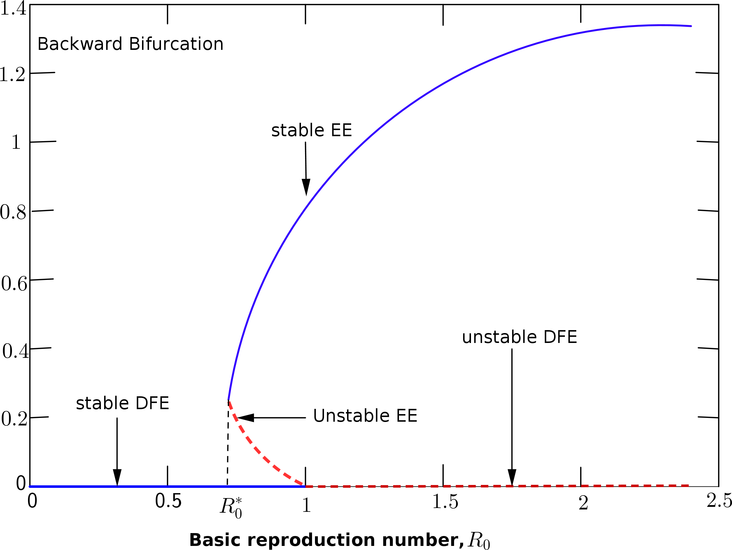
Figure 2. Description of the backward bifurcation of the model system (1) with \(\beta\) chosen as the bifurcation parameter.
Figure 2 depicts the qualitative backward bifurcation diagram which describe the behaviour of the reproduction number when equated to \(1\) and \(\beta\) chosen as the bifurcation parameter. The diagram shows that; if \(R_0\) is below unity then eradicating the disease depends on the size of the population under consideration. However, reducing the saddle node bifurcation value \(R_0^{*}\); which is obtained by setting the discriminant of the polynomial (13) to zero to obtain
\begin{align*}
R_0^{*} = 1 – \frac{\mathcal{U}_1^{2}}{4\mathcal{U}_2(\mu \mathcal{T}_1)(\mu\mathcal{T}_2 +\gamma_2 \mathcal{T}_3 +\gamma_1 \mathcal{T}_4)} ,
\end{align*}
where
\begin{align*}
\mathcal{T}_1 = (\theta + \mu+\omega), \quad \mathcal{T}_2 = (\alpha+\sigma+\mu+\rho), \quad \mathcal{T}_3 = (\sigma+\mu+\rho), \quad \mathcal{T}_4 = (\alpha+\mu+\gamma_2),
\end{align*}
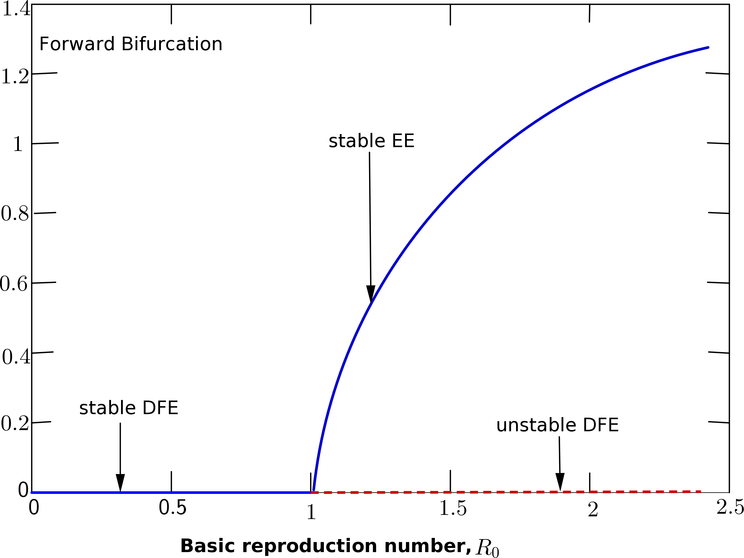
may result to controlling the disease. However, this can be guaranteed only when the disease-free equilibrium is globally asymptotically stable. For the backward bifurcation curve to disappear, there should be an increase in the efficacy rate of the vaccine given to individuals most importantly to a value say one. The biological meaning is that with an increase in the efficacy rate which corresponds with the disappearance of the backward bifurcation curve, lowering \(R_0 < 1\) will be sufficient to eliminate the disease from the population. Thus, \(R_0< 1\) would be sufficient to make the disease-free equilibrium globally stable. This is shown from the forward bifurcation curve in Figure 3.
Figure 3. Description of the forward bifurcation of system (1).
4. Numerical Simulation
We investigate the dynamics of system (1) numerically by using a set of reasonable approximate parameter values obtained from literature and tabulated in Table 1. The initial conditions are given by: \(S(0) = 380000\), \(V(0) = 100000\), \(I(0) = 10000\), \(C(0) = 10000\) and \(R(0) = 0\). The system was simulated using convenient programming language.
Table 1. Numerical values of parameters used for the simulation.
4.1. Numerical results in the presence of vaccination
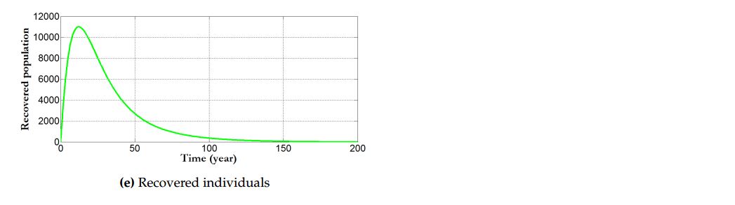
Here, we consider approximate values of important parameters to be able to predict the behaviour of the reproduction number of infection by considering the flow of the state variables. Figure 4 shows how the reproduction number \(R_0\) evolve with a vaccination rate \(\theta = 0.9\) and the efficacy rate of the vaccine at \(1\). We note that the presence of vaccination with a stronger efficacy decreases the reproduction number below unity and shows the importance of vaccination in the fight against HPV. With parameter values of \(\pi = 0.028\times 500000\), \(\beta = 0.8\), \(\theta = 0.9\), \(\eta = 0.3\), \(\epsilon = 1\), \(\omega = 0.3\), \(\sigma = 0.2\), \(\gamma_1 = 0.1\), \(\gamma_2 = 0.1\), \(\rho = 0.06\), \(\alpha = 0.03\) and \(\mu = 0.1\), we observe that the system settles at the disease-free state with \(R_0 = 0.8562\). At the disease-free state, the infectives tend to zero. However, due to recruitment of individuals into the susceptible population and the presence of individuals being vaccinated; the recovered population increases but the absence of infection means there will be no transmission of the disease and thus no recovery. The susceptible compartment shows a downward sloping curve. It shows the effect the presence of vaccination has on the number of susceptible individuals. A decrease in the number of susceptible individuals indicates that majority are vaccinated. However, the curve asymptotically approaches zero. The presence and application of vaccines causes the vaccinated individuals to increase. The curve of the vaccinated compartment slopes downward when the effectiveness or strength of the vaccine has been achieved for a period of time, say three years from Figure 4(b).
Figure 4. Simulation results of the behaviour of the state variables in the presence of vaccination which causes the model system to settle at the disease-free equilibrium state.
4.2 Effect of vaccination on infected and cancer population
Figure 5. Simulation results showing the effect of varying the vaccination rate; \((\theta)\), on (a) the infected individuals and (b) individuals with cancer population.
Figure 5 shows the changes that occurs in the population with time when vaccination is incorporated. It gives a clear indication on the role vaccination plays in reducing HPV in the population. Figure 5(a) shows the changes that occurs in the infected population while Figure 5(b) shows the changes that occurs in the population of individuals who progressed to develop cancer. It is notice from this figure that as the vaccination rate \((\theta)\) increases from \(0.3\), to \(0.7\) and further to \(0.9\), both the infected individuals as well as individuals who progress to develop cancer reduces as indicated by the blue, black and red lines respectively. This implies that majority of the individuals in the susceptible population have been vaccinated causing a reduction in the number of individuals who get infected with HPV.
4.3. Effect of waning vaccination on susceptible, infected and cancer population
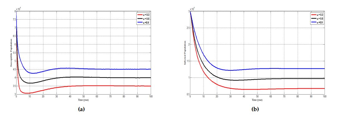
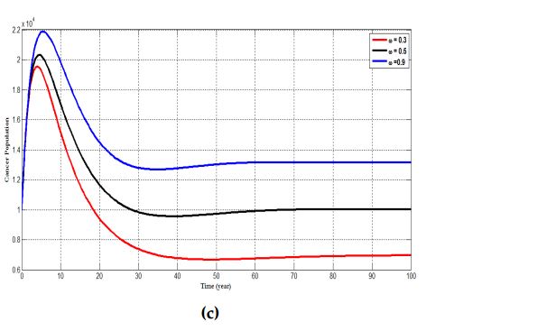
Figure 6. Simulation results showing the effect of varying the rate at which individuals wane their vaccine \((\omega)\) on (a) the susceptible individuals, (b) infected individuals and (c) individuals with cancer. The parameter \(\theta = 0.3, 0.5\) and \(0.9\) respectively represent the red, black and blue curve.
Figure 6, depicts the effect of what happens when an individual wanes their vaccine and further affirm the role vaccination plays in reducing the incidence of HPV infection in the population. A change or modification in the behaviour of an individual in the susceptible population leads to an increase in the chances of that individual being infected with HPV. It can be seen that for a waning rate of \(0.3\) there is a lower chance of an individual been infected with HPV. However, when the waning rate increases from \(0.3\) to \(0.9\), the chance of been infected also increases. Similarly, an increase in the rate at which an infected individual wane their vaccine leads to a higher probability of progressing to develop cervical cancer and vice versa. Furthermore, an individual with cancer who wanes their vaccine have a lower chance of getting treated and vice versa. Generally, as the waning rate increases the number of susceptible individuals who becomes infected as well as individuals who are infected progressing to develop cancer and those with cancer not being treated increases.
4.4. Variation of cancer population under different rate of \(\rho\)
For the given parameter values \(\beta =0.8\), \(\theta = 0.4\), \(\eta = 0.3\), \(\epsilon=0.7\), \(\sigma = 0.2\), \(\gamma_1 = 0.1\), \(\gamma_2 = 0.1\), \(\mu = 0.1\) and varying \(\rho\) (the number of individuals who receive cancer treatment), we determine the effect of \(\rho\) on the cancer compartment.
Figure 7. shows the changes in the number of individuals with cervical cancer for different values of the treatment rate \(\rho\).
Figure 7 tracks the changes in the population of individuals who progress to develop cervical cancer. If individuals with cancer are not treated, that is, when we set \(\rho = 0\), then the reproduction number increases and the endemic equilibrium population of these individuals also increases. However, when we increase the number of individuals who are treated say \(\rho = 0.1\), \(\rho = 0.3\) and \(\rho = 0.45\), we observe a decrease in the compartment of individuals with cervical cancer. This is because for a higher values of treatment there is a decrease in the available number of individuals with cervical cancer. However, the individuals with cancer begins to increase when the additions from the number of individuals who are infected with HPV start increasing.
4.5 Variation of infected population under different rate of \(\epsilon\)
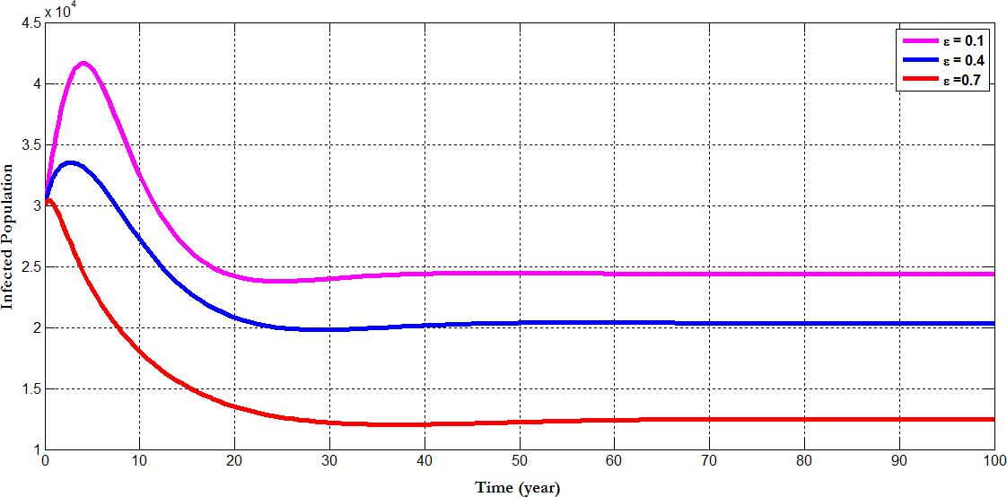
Figure 8 tracks the changes that occurs in the population of infected individuals with HPV using different efficacy rate; which shows the strength of the vaccine. For \(\epsilon=0.1\), we observe an increase in the number of individuals who are infected with HPV. However, when the efficacy rate of the vaccine is increased from \(0.1\) to \(0.4\) and further to \(0.7\), it is seen that the number of individuals in the infected population decreases; a situation which indicates that most individuals are been treated from the disease and this assertion is confirm from Figure 7 where an increase in the treatment rate \((\rho)\) corresponds with a decrease in the number of individuals who progress to develop cervical cancer.
Figure 8. shows the changes in the number of infected individuals for different values of \(\epsilon\).
4.6. Sensitivity analysis
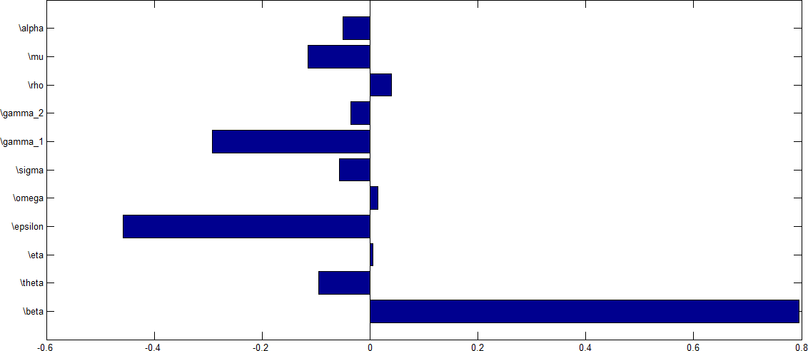
Sensitivity analysis was performed to determine parameters which contribute to the variability of the HPV infection using the reproduction number as an index case. To determine which parameter have high influence on the reproduction number, the partial Rank Correlation Coefficients (PRCCs) is performed to determine the sensitivity analysis for each parameter value sampled by the LHS scheme. The tornado plot for the normalised sensitivity index after performing a \(1000\) simulation run is shown in Figure 9.
Figure 10. shows tornado plot of PRCCs of parameters that influence \(R_0\) using values in Table \(\ref{tab}\).
From Figure 9, parameters with positive PRCCs will increase \(R_0\) when they are increased, while parameters with negative PRCCs will decrease \(R_0\) when they are increased. This implies that when the efficacy rate as well as individuals who receives vaccination are increase, the rate at which the disease will be transmitted from one individual to the other will decrease leading to a corresponding decrease in the value of \(R_0\). Similarly, an increase in the rate at which individuals wanes their vaccine as well as an increase in the transmission rate will increase the value of the rate of \(R_0\).
The contour plot in Figure 10 illustrate the relationship between the treatment rate \((\rho)\) and effective contact rate \((\beta)\). The figure shows a positive correlation between the transmission and treatment rate in the sense that, an increase in the transmission of the disease will call for more treatment of individuals who are infected and vice versa. This means that for a higher treatment rate, the number of individuals who are treated increases and thus the number of individuals with cervical cancer decreases. The results indicate that if no policy measures are put in place to control the transmission (effective) contact rate, the spread of the infection will lead to an increase in the number of individuals who are infected and subsequently leads to an increase in the number of individuals who progress to develop cervical cancer.
Figure 11. Contour plot showing the effect of parameters \(\beta\) and \(\rho\) on \(R_0\).
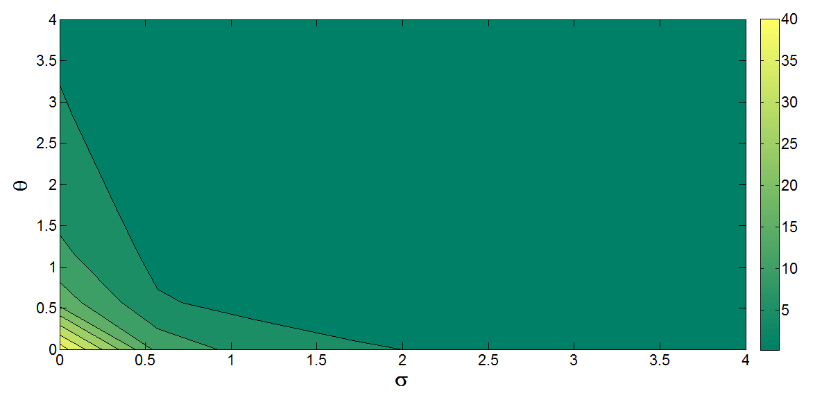
Similarly, from Figure 11, it is observe that the parameters \(\theta\) and \(\sigma\) have a negative correlation. This has to do with the fact that as more individuals receives vaccination, the tendency of those individuals progressing to develop cervical cancer decreases.
Figure 12. Contour plot for \(R_0\) as a function of \(\theta\) and \(\sigma\).
5. Discussion
In this paper, we analyzed a mathematical model for the transmission dynamics of HPV infection with vaccination as a control measure. Individuals who are susceptible are vaccinated and those who progress to develop cervical cancer undergo treatment. The reproduction number was used to ascertain the increase and decrease of infection among individuals in the population. Numerical results show that when we increase the proportion of individuals who are vaccinated, the reproduction number can be reduced below unity. Thus, \(R_0\) decreases with the vaccination rate indicating that, vaccination is useful in controlling the HPV infection. The basic reproduction number, \(R_0\), is directly proportional to the effective contact rate and indirectly proportional to the number of individuals who recover from cancer, those who die naturally and those who are vaccinated. The model system studied, however, indicated that \(R_0\) which happens to be the threshold is not enough to control the spread of HPV infection. This is because, the result of the stability analysis investigated show that the model exhibit a local asymptotic stability under certain conditions at the disease-free equilibrium provided \(R_0 < 1\) while the stability of the endemic equilibrium examined using the centre manifold theory proved the existence of a backward bifurcation phenomenon under certain conditions.
Sensitivity analysis performed on the parameters in the reproduction number show that parameters; \(\beta\), \(\eta\), \(\omega\) and \(\rho\), has a positive relationship while parameters; \(\alpha\), \(\mu\), \(\gamma_1\), \(\gamma_2\), \(\sigma\), \(\epsilon\) and \(\theta\) has a negative relationship with \(R_0\). The model system was observed to settle at the disease-free state when \(\epsilon=1\) and \(\theta\) (vaccination rate) having a value greater than \(0.4\). Thus, vaccination plays a key role in the attempt to help eradicate the transmission of HPV infection. Hence, it is important to incorporate vaccination as a control measure in the fight against cervical cancer due to HPV.
Although the eradication of HPV infection remains a challenge, the fact that cervical cancer is a preventable disease gives hope in the quest to help eradicate it. Based on the findings of this study, we suggest that effective vaccination control strategy should be included on governments HPV control programmes. Vaccines with strong efficacy should be used in order to reduce the transmission of HPV infection since vaccination has a greater impact on the reduction of the disease. However, this reduction also depends on the efficacy of the vaccine.
Acknowledgments
The authors thank the reviewers for for their useful comments, which led to the improvement of the content of the paper.
Author Contributions
All authors contributed equally to the writing of this paper. All authors read and approved the final manuscript.
Competing Interests
The author(s) do not have any competing interests in the manuscript.
References
Pongsumpun, P. (2014). Mathematical model of cervical cancer due to human papillomavirus infection. Mathematical Methods in Science and Engineering,ISBN: 978-1-61804-256-9. [Google Scholor]
Lee, S. L., & Tameru, A. M. (2012). A mathematical model of human papillomavirus (HPV) in the United States and its impact on cervical cancer. Journal of Cancer, 3, 262.[Google Scholor]
http://www.cancer.org/cancer/cervicalcancer/detailedguide/cervical-cancer-what-is-cervical-cancer (Accessed April 2016) [Google Scholor]
Clifford, G. M., Smith, J. S., Plummer, M., Munoz, N., & Franceschi, S. (2003). Human papillomavirus types in invasive cervical cancer worldwide: a meta-analysis. British journal of cancer, 88(1), 63-73.[Google Scholor]
Human Papillomavirus (HPV). Genetal HPV infection, cdc fact sheet, http://www.cdc.gov/std/hpv/stdfact-hpv.htm (Accessed April 2016) [Google Scholor]
Parkin, D. M., Laara, E., & Muir, C. S. (1988). Estimates of the worldwide frequency of sixteen major cancers in 1980. International journal of cancer, 41(2), 184-197. [Google Scholor]
Hughes, J. P., Garnett, G. P., & Koutsky, L. (2002). The theoretical population-level impact of a prophylactic human papilloma virus vaccine. Epidemiology, 13(6), 631-639. [Google Scholor]
Human Papillomavirus (HPV) Information center. Genetal HPV infection, cdc fact sheet, http://www.
hpvcentre.net/ (Accessed October 2017)[Google Scholor]
Bruni, L., Barrionuevo-Rosas, L., Albero, G., Aldea, M., Serrano, B., Valencia, S., … & Bosch, F. X. (2015). ICO information centre on HPV and cancer (HPV Information Centre). Human papillomavirus and related diseases in the world. Summary Report, 4(08). [Google Scholor]
Muller, H., & Bauch, C. (2010). When do sexual partnerships need to be accounted for in transmission models of human papillomavirus?. International journal of environmental research and public health, 7(2), 635-650. [Google Scholor]
Ribassin-Majed, L., Lounes, R., & Clémençon, S. (2012). Efficacy of vaccination against HPV infections to prevent cervical cancer in France: present assessment and pathways to improve vaccination policies. PLoS One, 7(3), e32251. [Google Scholor]
Llamazares, M., & Smith, R. J. (2008). Evaluating human papillomavirus vaccination programs in Canada: should provincial healthcare pay for voluntary adult vaccination?. BMC Public Health, 8(1), 114. Doi: 10.1186/1471-2458-8-114.[Google Scholor]
Shaban, N., & Mofi, H. (2014). Modelling the impact of vaccination and screening on the dynamics of human papillomavirus infection. International Journal of Mathematical Analysis, 8(9), 441-454. [Google Scholor]
Diekmann, O., Heesterbeek, J. A. P., & Metz, J. A. (1990). On the definition and the computation of the basic reproduction ratio R 0 in models for infectious diseases in heterogeneous populations. Journal of mathematical biology, 28(4), 365-382. [Google Scholor]
Castillo-Chavez, C., Feng, Z., & Huang, W. (2002). On the computation of $R_o$ and its role on. Mathematical approaches for emerging and reemerging infectious diseases: an introduction, 1, 229. [Google Scholor]
Li, M. Y., & Wang, L. (1998). A criterion for stability of matrices. Journal of mathematical analysis and applications, 225(1), 249-264.[Google Scholor]
Castillo-Chavez, C., & Song, B. (2004). Dynamical models of tuberculosis and their applications. Mathematical biosciences and engineering, 1(2), 361-404. [Google Scholor]
Nyabadza, F. (2006). A mathematical model for combating HIV/AIDS in Southern Africa: will multiple strategies work?. Journal of Biological Systems, 14 (03), 357-372. [Google Scholor]