Open Journal of Mathematical Sciences

Vol. 3 (2019), Issue 1, pp. 198 – 209
ISSN: 2523-0212 (Online) 2616-4906 (Print)
DOI: 10.30538/oms2019.0063

Transmission dynamics of two strain herpes simplex virus

Shamsuddeen Ibrahim$^1$, Nicholas Kwasi-Do Ohene Opoku, Hamenyimana Emanuel Gervas
Inspire Paradigm Academy Army Barracks Road, Jimeta, Yola North, Adamawa State, Nigeria.;(S.I)
African Institute for Mathematical Sciences, Ghana.; (S.I & N.K.O.O & H.E.G)
$^{1}$Corresponding Author: shamsuddeen@aims.edu.gh

Copyright © 2019 Shamsuddeen Ibrahim, Nicholas Kwasi-Do Ohene Opoku, Hamenyimana Emanuel Gervas. This is an open access article distributed under the Creative Commons Attribution License, which permits unrestricted use, distribution, and reproduction in any medium, provided the original work is properly cited.

Received: March 16, 2019 – Accepted: June 03, 2019 – Published: June 30, 2019

Abstract

A deterministic model for the transmission dynamics of two-strains Herpes Simplex Virus (HSV) is developed and analyzed. Following the qualitative analysis of the model, reveals a globally asymptotically stable disease free equilibrium whenever a certain epidemiological threshold known as the reproduction number ($\mathcal{R}_0$), is less than unity and the disease persist in the population whenever this threshold exceed unity. However, it was shown that the endemic equilibrium is globally asymptotically stable for a special case. Numerical simulation of the model reveals that whenever $\mathcal{R}_1<1<\mathcal{R}_2$, strain 2 drives strain 1 to extinction (competitive exclusion) but when $\mathcal{R}_2<1<\mathcal{R}_1$, strain 1 does not drive strain 2 to extinction. Finally, it was shown numerically that super-infection increases the spread of HSV-2 in the model.

Keywords:

HSV strains, equilibria, stability.

1. Introduction

Herpes simplex virus (HSV) is a kind of infection that causes herpes. Herpes can appear in different part of the body, particularly on the mouth or genital area. HSV infections are endemic throughout the world[1, 2, 3, 4, 5]. For both point-prevalence and prospective studies, a large percentage of persons that are seropositive for HSV type 1 (HSV-1) or HSV type 2 (HSV-2) have no clinical manifestations of the disease [1, 2, 3, 4, 5,6]. HSV-1 and HSV-2 are lifelong infections [1, 2]. HSV-1 is mainly transmitted by oral to oral contact to cause infection in or around the mouth (oral herpes). HSV-2 is almost exclusively sexually transmitted, causing infection in the genital or anal area (genital herpes). Nonetheless, HSV-1 can also be transmitted to the genital area through oral-genital contact to cause genital herpes [2].

In $2012$, it was estimated that about 3.7 billion people under the age of $50$, or $67\%$ of the population had HSV-1 infection while over $267$ million women and $150$ million men were living with HSV-2 infection [2]. Estimated prevalence of HSV-1 infection was highest in Africa, $87\%$ and lowest in the Americas $40-50\%$ [2]. Prevalence of HSV-2 infection was estimated to be highest also in Africa $(31.5\%)$, followed by the Americas $(14.4\%)$ [2, 7]. This is a clear sign that there should be a global call to fight against the global burden of HSV.

Many mathematical models have been developed to study the dynamics of HSV-2 see [8, 9, 10, 11, 12,13,14, 15]. In the manner that, Sally Blower and Li ma [13] formulated a mathematical model that predicts the effect of high prevalence of HSV-2 on HIV. Their results showed that HSV-2 epidemic has more than double impact on the peak of HIV incidence. Abu-Raddad et al [16], considered a homosexual male population and suggested that HSV-2 prevalence, if near endemic level may predict the spread of HIV. Foss et al. [17], developed a dynamical model to estimate the HIV infection due to HSV-2 in heterosexual population. Alvey et al. [18], developed a model that takes into account the transmission through either homosexual or heterosexual behaviour and investigate the impact of the coupled dynamics of HIV and HSV-2. Their results showed that homosexual transmission has great impact on the disease prevalence.

For all the models considered so far and to the best of our knowledge, none of them considered the transmission dynamics of the two strain of HSV. However, a detailed study of the transmission dynamics of disease with multiple strains has been one of the important problems in epidemiology. Hence, in order to fight against this global socio-economic burden, a deterministic model of two strains of HSV is developed and rigorously analysed, to get more insight into the long-term dynamics of the disease.

The paper is organized as follows. The model is formulated in Section 2 while it is analysed in Section 3. Also the numerical simulation is presented in Section 4 and the conclusion is drawn in Section 5.

2. Model formulation

The model is based on the transmission dynamics of HSV. The total population at time $t$ is denoted by $N(t)$. This is divided into susceptible individuals $S(t)$; infectious individuals infected with strain $1$ $I_1(t)$, infectious individuals infected with strain $2$~ $I_2(t)$; such that $$N(t)=S(t)+I_1(t)+I_2(t).$$ We give the detailed explanation of the transmission in the schematic diagram below:

Figure 1. Schematic diagram of the two strain HSV epidemic model with superinfection and the arrows with head indicate movement.

It is assumed that the susceptible population is generated at a constant rate $\wedge$. It is reduced due to infection by either HSV-1 (at a rate $\beta_1$) or by HSV-2 (at a rate $\beta_2$) and natural death at a rate $\mu$, such that $$\frac{dS}{dt}=\wedge-\beta_1S I_1 -\beta_2 SI_2 -\mu S.$$ The rate of change of the infectious individuals infected with strain $1$ is increased by infecting the susceptible population (at a rate $\beta_1$). It is decreased due to genital herpes induced by HSV-1 (at a rate $\eta$) and by natural death (at a rate $\mu$), so that $$\frac{dI_1}{dt}=\beta_1S I_1 -\left(\eta+\mu\right)I_1.$$ Finally, the rate of change of the infectious individuals infected with strain $2$ is increased by infecting the susceptible population (at a rate $\beta_2$) and due to genital herpes induced by HSV-1 (at a rate $\eta$). It is decreased due natural death (at a rate $\mu$). Thus $$\frac{dI_2}{dt}=\beta_2 SI_1+ \eta I_1-\mu I_2.$$ In summary, the model for the transmission dynamics of both HSV-1 and HSV-2 is given by the non-linear differential equations. The model variables and parameters are described in 1 and the schematic diagram of the model is depicted in Figure 1.

\begin{equation}\label{sham} \begin{split} \frac{dS}{dt}&=\wedge-\beta_1S I_1 -\beta_2 SI_2 -\mu S\\ \frac{dI_1}{dt}&=\beta_1S I_1 -\left(\eta+\mu\right)I_1\\ \frac{dI_2}{dt}&=\beta_2 SI_1+ \eta I_1-\mu I_2 \end{split} \end{equation}

(1)

Table 1. Description of model variables and parameters.

Variables	Description
$S(t)$	Susceptible Population
$I_1(t)$	Individuals infected with strain 1
$I_2(t)$	Individuals infected with strain 2
$\wedge$	Recruitment rate
$\beta_1$	Efficient contact rate of strain 1
$\beta_2$	Efficient contact rate of strain 2
$\eta$	Rate of genital herpes induced by strain 1
$\mu$	Natural mortality rate

2.1. Basic properties of the model

For the model to be epidemiologically meaningful, we need to prove that all the states variables are non-negative for all time $t$. In other words the solution of Equation (1) with positive initial condition will remain positive for all $t\geq 0$.

Theorem 1. If the initial condition $S(0)>0$, $I_1(0)>0$ and $I_2(0)>0$, then the solutions $S$, $I_1$, and $I_2$ of model Equation (1) are positive for all $t$.

Proof. Given that $S(0)>0$, $I_1(0)>0$ and $I_2(0)>0$, we want to show that $S(t)>0$, $I_1(t)>0$ and $I_2(t)>0$. Let $\tau=\text{sup}\left\{t>0: S(t)>0, I_1(t)>0, I_2(t)>0\right \}$. Thus $\tau >0$. Lets consider the first equation in Equation (1), we have that

\begin{align}\label{s2} \frac{dS}{dt}\geq -\left(\phi(t)+\mu\right)S,~~~\mbox{where $\phi(t)=\beta_1 I_1(t)+\beta_2 I_2(t)$}. \end{align}

(2)

Integrating the above equation, we get

\begin{align}\label{s3} S(\tau)\geq S(0)e^{\left\{-\left[\int^{\tau}_{0}\phi(t)dt +\mu \tau\right]\right\}}. \end{align}

(3)

Considering the second equation in Equation (1), we have that

\begin{align}\label{s4} \frac{dI_1}{dt}\geq -\left(\eta+\mu\right)I_1. \end{align}

(4)

Integrating the above equation, we get

\begin{align}\label{s5} I_1(\tau)\geq I_1(0)e^{-\left(\eta+\mu\right)\tau}. \end{align}

(5)

Finally, considering the third equation in Equation (1), we have that

\begin{align}\label{s6} \frac{dI_2}{dt}\geq -\mu I_2. \end{align}

(6)

Integrating the above equation, yields

\begin{align}\label{s7} I_2(\tau)\geq I_2(0)e^{-\mu \tau}. \end{align}

(7)

Thus $S(t)$, $I_1(t)$ and $I_2(t)$ are all positive for any non-negative initial conditions.

2.2. Positively invariant region

Lemma 2. The region $$\Gamma=\left\{\left( S,I_1,I_2\right) \in \mathbb{R}^{3}_{+}: S+I_1+I_2\leq \frac{\wedge}{\mu}\right \} $$ is positively invariant and attracting in Equation (1).

Proof. Adding the Equation (1), gives \begin{align*} \frac{dN}{dt}&=\wedge-\mu\left(S+I_1+I_2\right),\\ \frac{dN}{dt}&\leq\wedge-\mu N. \end{align*} Thus the population is bounded above by $\frac{\wedge}{\mu}$ so that $\frac{dN}{dt}< 0$ whenever $N(t)>\frac{\wedge}{\mu}$. Hence by comparison Theorem [19], $N(t)\leq N(0)e^{-\mu t}+\frac{\wedge}{\mu}\left[1-e^{-\mu t}\right]$, in particular $N(t)\leq \frac{\wedge}{\mu}$ if $N(0)\leq \frac{\wedge}{\mu}$. Thus, $\Gamma$ is positively invariant. Also if $N(0)>\frac{\wedge}{\mu}$, then either the solution enters $\Gamma$ in finite time or $N(t)$ approaches $\frac{\wedge}{\mu}$ asymptotically. Therefore, the region $\Gamma $ attracts all solution in $\mathbb{R}^{3}_{+}$. Hence, it suffices to consider the dynamics of the model Equation (1) in $\Gamma$, where the model is epidemiologically and mathematically well posed [20].

3. Model analysis

3.1. Disease-free equilibrium point

At equilibrium point, we equate each of the right hand side of Equation (1) to zero and solve. Where we represent diseases free equilibrium (DFE) as $E_0$ to be

\begin{equation}\label{s8} E_0 =\left(S^0,I^{0}_1, I^{0}_2\right)=\left(\frac{\wedge}{\mu},0,0\right). \end{equation}

(8)

3.2. Basic reproduction number ($\mathcal{R}_0$)

The basic reproduction number $\mathcal{R}_0$ measures the average number of secondary new infections caused by one primary infection in a completely susceptible population. $\mathcal{R}_0$ gives the threshold whether a disease will go extinction or persist. In this research, we find our $\mathcal{R}_0$ using the next generation matrix method on Equation (1). Using the notation in [21], the matrices $\mathscr{F}$ is the rate of appearance of new infections in compartment $i$, and $\mathscr{V}$ is the rate of other transitions between compartment $i$ and other infected compartments of Equation (1) are given respectively by \begin{equation*} \mathscr{F}= \begin{bmatrix} \beta_1SI_1\\ \beta_2SI_2+\eta I_1 \end{bmatrix}, \end{equation*} \begin{equation*} \mathscr{V}= \begin{bmatrix} \left(\eta +\mu\right)\mu\\ \mu I_2 \end{bmatrix}. \end{equation*} Computing the matrices $F$ and $V,$ for the new infection terms and of the transition terms, respectively, we have \begin{equation*} F= \begin{bmatrix} \frac{\beta_1 \wedge}{\mu}&0\\ \eta& \frac{\beta_2 \wedge}{\mu} \end{bmatrix}, \end{equation*} \begin{equation*} V= \begin{bmatrix} \eta +\mu&0\\ 0& \mu \end{bmatrix}. \end{equation*} Thus, the basic reproduction number of Equation (1), denoted by $\mathcal{R}_0$, is given by (where $\rho$ is the spectral radius) \begin{equation*} \mathcal{R}_0=\rho\left(FV^{-1}\right)=\text{max}\left\{\mathcal{R}_{1},\mathcal{R}_{2}\right\}, \end{equation*} where $\mathcal{R}_{1}$ and $\mathcal{R}_{2}$ are the associated reproduction numbers of strain $1$ and strain $2$, respectively given by

\begin{equation}\label{s10} \mathcal{R}_{1}=\frac{\beta_1 \wedge}{\mu\left(\eta +\mu\right)}~~\text{and}~~ \mathcal{R}_{2}=\frac{\beta_2 \wedge}{\mu^2}. \end{equation}

(9)

3.3. Local stability of disease-free equilibrium

Theorem 3. The DFE of Equation (1), given by $E_0$, is locally asymptotically stable (LAS) if $\mathcal{R}_0< 1$, and unstable if $\mathcal{R}_0>1$.

Proof. The Jacobian matrix of Equation (1) denoted by $J$ is given as

\begin{equation}\label{s11} J= \begin{bmatrix} -\left(\beta_1 I_1+\beta_2 I_2+\mu\right)&-\beta_1 S&-\beta_2 S\\ \beta_1 I_1& \beta_1 S-\left(\eta+\mu \right)&0\\ \beta_2 I_2& \eta& \beta_2S-\mu \end{bmatrix}, \end{equation}

(10)

evaluating $J$ at $E_0$, we get \begin{equation*} J_{\left(\frac{\wedge}{\mu},0,0\right)}= \begin{bmatrix} -\mu&-\frac{\beta_1 \wedge}{\mu}&-\frac{\beta_2 \wedge}{\mu}\\ 0& \frac{\beta_1 \wedge}{\mu}-\left(\eta +\mu\right)&0\\ 0& \eta& \frac{\beta_2 \wedge}{\mu}-\mu \end{bmatrix}. \end{equation*} The eigenvalues associated with the above matrix are \begin{align*} \lambda_1&= -\mu,\\ \lambda_2&=\frac{1}{\mu}\left(\beta_1 \wedge-\eta \mu-\mu^2\right),\\ \lambda_3&= \frac{1}{\mu}\left(\beta_2 \wedge -\mu^2\right). \end{align*} But $\lambda_2$ and $\lambda_3$ can be re-written as $\left(\wedge+\mu\right)\left(\mathcal{R}_{1}-1\right)$ and $\frac{1}{\mu}\left(\mathcal{R}_{2}-1\right)$ respectively. It is clear that since $\lambda_1< 0$, then $E_0$ is LAS if $\lambda_2< 0$ and $\lambda_3< 0$ i.e if $\mathcal{R}_{1}< 1$ and $\mathcal{R}_{2}< 1$. And unstable if $\mathcal{R}_{01}>1$,$\mathcal{R}_{2}>1$ or both $\mathcal{R}_{1}$, $\mathcal{R}_{2}$ $>0$.

3.4. Global stability of disease-free equilibrium

Theorem 4. The DFE given by $E_0$ is globally asymptotically stable (GAS) in $\Gamma$ whenever $\mathcal{R}_{0}\leq 1$.

Proof. Consider the Lyapunov function for Equation (1)

\begin{equation}\label{s12} \mathcal{F}=K_1I_1+K_2 I_2, \end{equation}

(11)

Clearly the function $\mathcal{F}$ is continuous and positive definite, with lyapunov derivative given below $$\dot{\mathcal{F}}=K_1\dot{I_1}+K_2\dot{I_2}.$$ Substituting $\dot{I_1}$ and $\dot{I_2}$ in the above equation, we get

\begin{equation}\label{s13} \begin{split} \dot{\mathcal{F}}&=K_1\dot{I_1}+K_2\dot{I_2}\\ &= K_1\left[\beta_1 SI_1-\left(\mu+\eta\right)I_1\right] +K_2\left[\beta_1SI_2+\eta -\mu I_2\right]\\ &=K_1I_1\left[\beta_1 S-\left(\mu+\eta\right)\right]+K_2I_2\left[\beta_2 S-\mu\right]+K_2\eta I_1\\ &\leq K_1I_1\left[\frac{ \beta_1 \wedge}{\mu \left(\mu+\eta\right)}-1\right]+\mu K_2 I_2\left[\frac{\beta_2 \wedge}{\mu^2}-1\right]+ \eta I_1\left(\frac{\beta_1 \wedge}{\mu+\eta}-\mu\right)^2\\ &= K_1I_1\left[\mathcal{R}_{1}-1\right]+\mu K_2 I_2\left[\mathcal{R}_{2}-1\right]+ \mu^2\eta I_1\left[\mathcal{R}_{1}-1\right]^2\\ &=\left(\mu \eta +\beta_1 \beta_2\right)^4I_1\left[\mathcal{R}_{1}-1\right]+\mu^2\eta I_1\left[\mathcal{R}_{1}-1\right]^2+\mu I_2\left(\frac{\beta_1 \wedge}{\mu+\eta}-\mu\right)^2 \left[\mathcal{R}_{2}-1\right] \end{split}, \end{equation}

(12)

where $$K_1=\left(\mu \eta +\beta_1 \beta_2\right)^4 ~~\text{and}~~K_2=\left(\frac{\beta_1 \wedge}{\mu+\eta}-\mu\right)^2.$$ Thus from Equation (13), $\dot{\mathcal{F}}\leq 0$ if $\mathcal{R}_{0}=\text{max}\left\{\mathcal{R}_{1},\mathcal{R}_{2}\right\}\leq 1$ and $\dot{\mathcal{F}}=0$ if and only if $I_1=I_2=0.$ Substituting $I_1=I_2=0$ in Equation (1) we get $S(t)\to \frac{\wedge}{\mu} ~~\text{as}~~ t\to \infty$. Also the largest compact invariant set in $\left\{\left( S,I_1,I_2\right)\in \Gamma: \frac{d\mathcal{F}}{dt}=0\right\}$ is the singleton $\left\{E_0\right\}.$ Hence it follows from the Laselle invariance principle [22], every solutions in Equation (1) with initial condition in $\mathbb{R}^{3}_{+}$, converges to DFE $E_0$ as $t\to \infty$ whenever $\mathcal{R}_{0}=\text{max}\left\{\mathcal{R}_{1},\mathcal{R}_{2}\right\}\leq 1$. Thus the DFE, $E_0$, is GAS in $\Gamma$ for $\mathcal{R}_{0}=\text{max}\left\{\mathcal{R}_{1},\mathcal{R}_{2}\right\}\leq 1$.

3.4.1. Existence of endemic equilibrium

Finding the condition(s) for the existence of an equilibrium $E_* =\left(S^{*},I^{*}_1, I^{*}_2\right)$ of the model Equation (1) such that the disease is endemic in the population, the Equation (1) are solved at steady state which yields

\begin{equation}\label{s9} E_* =\left(\frac{\eta +\mu}{\beta_1},\frac{\beta_1 \mu I^{*}_{2}}{\left(\beta_2\left(\eta +\mu\right)+\beta_1\mu\right)},\frac{\left(\beta_2\left(\eta+\mu\right)\beta_1 \mu\right)\left(\beta_1\wedge-\mu\left(\eta +\mu\right)\right)}{\left(\eta+\mu\right)\left[\beta^{2}_{1}\mu+\beta^{2}_{2}\left(\eta +\mu\right)+\beta^{2}_{1}\beta^{2}_{2}\mu\right]}\right). \end{equation}

(13)

3.5. Local stability of endemic equilibrium

Theorem 5. The EE, $E_1$ of Equation (1) is LAS provided that

\begin{equation}\label{s14} q_1> q_2, \end{equation}

(14)

\begin{equation}\label{s15} q_3> q_4, \end{equation}

(15)

\begin{equation}\label{s16} q_5> q_6, \end{equation}

(16)

where $q_1$, $q_2$, $q_3$, $q_4$, $q_5$, and $q_5$ are given in the proof.

Proof. The characteristics polynomial of Equation (10) at $E_1$ can be written as

\begin{equation}\label{s17} \lambda^3+a_1 \lambda^2+a_2\lambda+a_3 =P(\lambda), \end{equation}

(17)

where

\begin{equation}\label{s18} \begin{split} a_1&=q_1-q_2,\\ a_2&=q_3-q_4,\\ a_3&=q_5-q_6,\\ \end{split} \end{equation}

(18)

with

\begin{equation}\label{s19} \begin{split} q_1&= \beta_1 I^{*}_1 +\beta_2 I^{*}_2+\left(\eta+3\mu\right),\\ q_2&=S^{*}\left(\beta_1+\beta_2\right),\\ q_3&=\beta_1 I^{*}_1\left(\eta+2\mu\right)+\beta_2 I^{*}_2\left(\eta+2\mu\right)+S^{*}\beta_1 \beta_2 +\mu\left(2\eta+3\mu\right),\\ q_4&=S^{*}\beta_1 \beta_2\left(I^{*}_1+I^{*}_2\right)+2S^{*}\mu \left(\beta_1+ \beta_2\right)+S^{*}\beta_2\eta,\\ q_5&=I^{*}_1\beta_1\mu\left(\eta+\mu\right)+I^{*}_2\beta_2\mu\left(\eta+\mu\right)+(S^{**})^2 \beta_1 \beta_2\mu +\mu\left(\eta+\mu^2\right),\\ q_6&=S^{*}\beta_1 \beta_2\left(I^{*}_1+I^{*}_2\right)+S^{*}\beta_1\mu^2+S^{*}\beta_2\mu\left(\eta+\mu\right). \end{split} \end{equation}

(19)

Under the conditions in Equation (14), (15), (16) and (17), $a_1>0$, $a_2>0$ and $a_3>0$. But $a_1 a_2=q_1q_3+q_2q_4-q_1q_4-q_2q_3$ and $a_1 a_2>a_3$ if $q_1q_3+q_2q_4-q_1q_4-q_2q_3>q_5-q_6$ that is if

\begin{equation}\label{s20} q_1q_3+q_2q_4+q_6>q_1q_4+q_2q_3+q_5. \end{equation}

(20)

Thus by the Routh- Hurwitz criterion [23] all the eigenvalues of Equation (10) at $E_1$ have negative real part. Hence the endemic equilibrium of Equation (1) subject to the conditions of Equation (14), (15), (16) ,(17) and (20) is LAS.

3.6. Global stability of endemic equilibrium: special case

Theorem 6. If $\mathcal{R}_{0}=\text{max}\left\{\mathcal{R}_{1},\mathcal{R}_{2}\right\}\geq1$ and $\eta=0$, then the endemic equilibrium is globally asymptotically stable (GAS) in $\Gamma$.

Proof. Consider the non-linear Lyapunov function (such non-linear functions has been used in many mathematical epidemiology, see [24, 25, 26, 27] for

\begin{equation} \mathcal{F}=S-S^{*}-S^{*}\ln\frac{S}{S^{*}}+I_1-I^{*}_1-I^{*}_1\ln\frac{I_1}{I^{*}_1}+I_2-I^{*}_2-I^{*}_2\ln\frac{I_2}{I^{*}_2}, \end{equation}

(21)

\label{s21} with Lyapunov derivative $$\dot{\mathcal{F}}=\dot{S}-\frac{S^{*}}{S}\dot{S}+\dot{I_1}-\frac{I^{*}_1}{I_1}\dot{I_1}+\dot{I_2}-\frac{I^{*}_2}{I_2}\dot{I_2}.$$ Substituting $\dot{S}$, $\dot{I_1}$ and $\dot{I_2}$ in the above equation, we get

\begin{equation}\label{s22} \begin{split} \dot{\mathcal{F}}&=\left[1-\frac{S^*}{S}\right]\left(\wedge-\beta_1S I_1 -\beta_2 SI_2-\mu S\right)\\&+\left[1-\frac{I^{*}_1}{I_1}\right]\left(\beta_1S I_1-\mu I_1\right)+\left[1-\frac{I^{*}}{S}_2\right]\left(\beta_2 SI_2-\mu I_2\right).\\ \end{split} \end{equation}

(22)

\text{It can be shown from Equation (1) with $\eta=0$, at endemic state that} \begin{align}\label{w1} \wedge&=\beta_1I^{*}_1S^*+\beta_2I^{*}_2S^*+\mu S^*, %\mu I^{*}_1&=\beta_1I^{*}_1S^*\\ %\mu I^{*}_2&=\beta_2I^{*}_2S^* \end{align} substituting Equation (23) into (22), we have

\begin{equation}\label{s23} \begin{split} \dot{\mathcal{F}}&=-\mu\frac{\left(S-S^*\right)^2}{S} +\beta_1S^*I^{*}_1\left(1-\frac{S^*}{S}\right)+\beta_2S^*I^{*}_2\left(1-\frac{S^*}{S}\right)+\beta_1SI_1\left(1-\frac{S^*}{S}\right)\\&+\beta_2SI_2\left(1-\frac{S^*}{S}\right)+\beta_1SI_1\left(1-\frac{I^{*}_1}{I_1}\right)-\mu I_1\left(1-\frac{I^{*}_1}{I_1}\right)+\beta_2SI_2\left(1-\frac{I^{*}_2}{I_2}\right)\\&-\mu I_2\left(1-\frac{I^{*}_2}{I_2}\right)\\ &=-\mu\frac{\left(S-S^*\right)^2}{S} +\beta_1S^*I^{*}_1-\frac{\beta_1 {S^{*}}^2 I^{*}_1}{S} +\beta_2S^*I^{*}_2-\frac{\beta_1 {S^{*}}^2 I^{*}_2}{S}+\beta_1S^*I_1+\beta_2S^*I_2\\&-\beta_1SI^{*}_1-\beta_2SI^{*}_2-\mu I_1+\mu I^{*}_1-\mu I_2+\mu I^{*}_2. \end{split} \end{equation}

(23)

\text{It can be shown from Equation (1) with $\eta=0$, at endemic state that}

\begin{equation}\label{24} \begin{split} \mu I^{*}_1&=\beta_1I^{*}_1S^*,\\ \mu I^{*}_2&=\beta_2I^{*}_2S^*. \end{split} \end{equation}

(24)

substituting Equation (25) into (24), we have

\begin{equation}\label{s25} \begin{split} \dot{\mathcal{F}}&=-\mu\frac{\left(S-S^*\right)^2}{S} +2\beta_1S^*I^{*}_1-\frac{\beta_1 {S^{*}}^2 I^{*}_1}{S} -\beta_1SI^{*}_1 +2\beta_2S^*I^{*}_2-\frac{\beta_2 {S^{*}}^2 I^{*}_2}{S} -\beta_2SI^{*}_2 \\ &+\beta_1S^*I_1-\mu I_1 +\beta_2S^*I_2-\mu I_2\\ &=-\mu\frac{\left(S-S^*\right)^2}{S} +2\beta_1S^*I^{*}_1-\frac{\beta_1 {S^{*}}^2 I^{*}_1}{S} -\beta_1S^*I^{*}_1\frac{S}{S^*} +2\beta_2S^*I^{*}_2-\frac{\beta_2 {S^{*}}^2 I^{*}_2}{S} \\&-\beta_2S^*I^{*}_2\frac{S}{S^*} +\beta_1S^*I_1-\frac{\mu I_1I^{*}_1}{I^{*}_1} +\beta_2S^*I_2-\frac{\mu I_2I^{*}_2}{I^{*}_2}\\ &=-\mu\frac{\left(S-S^*\right)^2}{S}+\beta_1S^*I^{*}_1\left(2-\frac{S^*}{S}-\frac{S}{S^*}\right)+\beta_2S^*I^{*}_2\left(2-\frac{S^*}{S}-\frac{S}{S^*}\right)+\beta_1S^*I_1\\&-\frac{\mu I_1I^{*}_1}{I^{*}_1}+\beta_2S^*I_2-\frac{\mu I_2I^{*}_2}{I^{*}_2}.\\ \end{split} \end{equation}

(25)

from Equation (25), we have (26) to be

\begin{equation}\label{s26} \begin{split} \dot{\mathcal{F}}&=-\mu\frac{\left(S-S^*\right)^2}{S}+\beta_1S^*I^{*}_1\left(2-\frac{S^*}{S}-\frac{S}{S^*}\right)+\beta_2S^*I^{*}_2\left(2-\frac{S^*}{S}-\frac{S}{S^*}\right)+\beta_1S^*I_1\\&-\frac{\beta_2 S^* I_1I^{*}_1}{I^{*}_1}+\beta_2S^*I_2-\frac{\beta_2 S^* I_2I^{*}_2}{I^{*}_2}\\ &=-\mu\frac{\left(S-S^*\right)^2}{S}+\beta_1S^*I^{*}_1\left(2-\frac{S^*}{S}-\frac{S}{S^*}\right)+\beta_2S^*I^{*}_2\left(2-\frac{S^*}{S}-\frac{S}{S^*}\right).\\ \end{split} \end{equation}

(26)

Since the arithmetic mean is greater than or equal to the geometric mean, then \begin{equation*} \begin{split} 2-\frac{S^*}{S}-\frac{S}{S^*}&\leq 0. \end{split} \end{equation*} Clearly, the first term of $\dot{\mathcal{F}}$ is always negative and the second and third terms are also negative, therefore $\dot{\mathcal{F}}\leq 0,$ with $\dot{\mathcal{F}}=0$ if and only if $S^*=S$. Also the largest compact invariant set in $\left\{\left( S,I_1,I_2\right)\in \Gamma: \frac{d\mathcal{F}}{dt}=0\right\}$ is the singleton $\left\{E_1\right\}.$ Thus by the Laselle Invariance Principle [22], every solutions in Equation (1) with initial conditions in $\mathbb{R}^{3}_{+}$, converges to $E_1$ as $t\to \infty$ whenever $\mathcal{R}_{0}=\text{max}\left\{\mathcal{R}_{1},\mathcal{R}_{2}\right\}\geq 1$. Hence, $E_1$, is GAS in $\Gamma$ for $\mathcal{R}_{0}=\text{max}\left\{\mathcal{R}_{1},\mathcal{R}_{2}\right\}> 1$.

4. Numerical simulations and discussions

In this section, the model Equation (1), using the parameter values given in Table 2 (unless otherwise stated), to assess the impact of super-infection on the dynamics of two strain HSV. The objective of this section is to illustrate some of the theoretical results in this paper. Since the model presented in this paper is completely new (no similar two strain model for HSV model has yet been published in the literature to our knowledge), appropriate data for estimating the associated parameters are not available at the present time. Thus, the parameter values chosen for the numerical simulations below may not all be realistic biologically, although such uncertainties in parameter values are partially addressed below by considering different rate of genital herpes induced by strain 1(super-infection) in the simulations, it is important to emphasize that the simulation results obtained should be interpreted bearing these uncertainties in mind.

Table 2. Parameter values for model Equation (1).

Parameters	Baseline value	Reference
$\wedge$	10000 per day	Assumed
$\beta_1$	$7\times 10^{-9}$ per day	Assumed
$\beta_2$	$2\times 10^{-9}$ per day	Assumed
$\eta$	$0.0022$ per day	Assumed
$\mu$	$0.0167$ per day	Assumed

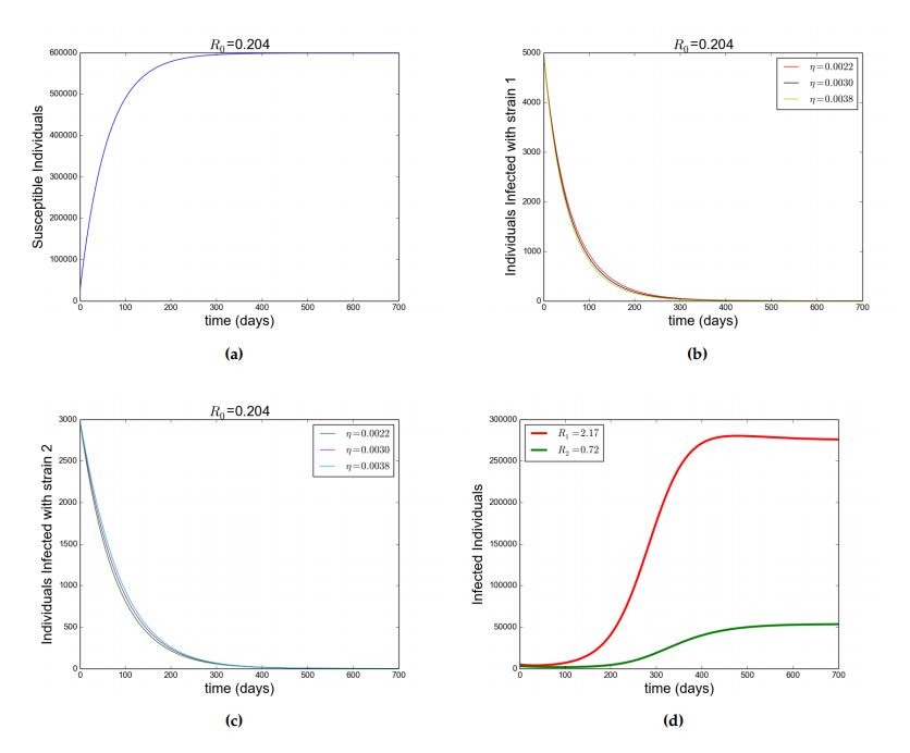
With the given parameters in Table 2, $\mathcal{R}_{1}=0.204$ and $\mathcal{R}_{2}=0.072$ such that $\mathcal{R}_{0}=0.204< 1$. It is observed that the susceptible individuals increases as a result $\wedge$ which is the recruitment rate, however due to natural mortality rate $\mu$ the increase in susceptible individuals is regulated, moreover individuals in the susceptible compartment reach a saturation point $600000$ ($\frac{\wedge}{\mu}$) from Figure (2a). This shows that as time increases the individuals who enter the susceptible compartment would equal to those who leave the compartment as a result of natural mortality rate $\mu$. It was also observed that whenever there is no disease Figure (2b) and (2c) goes to zero. Therefore by Theorem 4 the DFE is GAS. Figure (2a), (2b) and (2c) shows this this simulations, confirming the GAS property of the DFE. In addition, the effect of super-infection governed by $\eta$ is monitored, which shows that the total number of infected individuals with strain $2$ increases with increase in $\eta$ and decreases with decrease in $\eta$. This is depicted in Figure (2b) and (2c). Furthermore, in Figure (2d) and (3), additional simulation shows that when $\mathcal{R}_{2}< 1< \mathcal{R}_{1}$, strain $1$ does not drive strain $2$ to extinction but when $\mathcal{R}_{1}< 1< \mathcal{R}_{2}$, strain $2$ drives out strain $1$ to extinction (competitive exclusion).

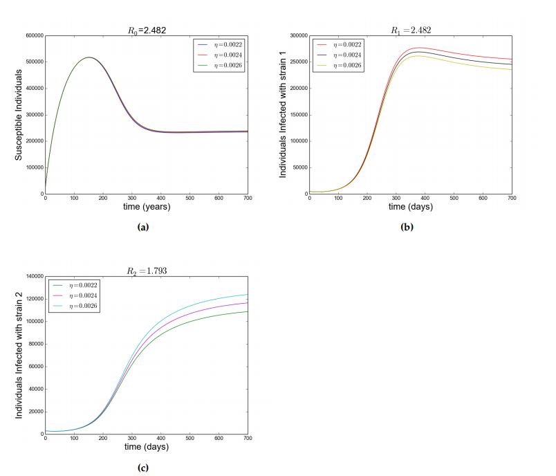
Figure (4a) depicts the scenario where the susceptible individuals increases then decreases but stabilizes in the system as a result of $\mathcal{R}_{0}>1$ and Figure (4b) and (4c) shows how individuals infected with srain $1$ and strain respectively evolve due to $\mathcal{R}_{0}>1$. Also, Figure (4b) and (4c) shows that when $\mathcal{R}_{1}>1$ and $\mathcal{R}_{2}>1$, strain $1$ and strain 2 co-exist.

Figure 2. Showing simulation of model Equation (1). Figure (a), (b) and (c) shows how the susceptible individuals, infected individuals with strain $1$ and infected individuals with strain $2$ respectively evolve when $\mathcal{R}_0< 1$ with parameters as in Table 2. (d) $\mathcal{R}_2< 1 < \mathcal{R}_1$ with $\beta_1=7\times 10^{-8},~\beta_2=2\times 10^{-8}$. Other parameters as in Table 2 and different values of $\eta$ as in legend.

Figure 3. Showing simulation of model Equation (1), $\mathcal{R}_1< 1< \mathcal{R}_2$ with $\beta_1=2\times 10^{-8},~\beta_2=7\times 10^{-8}$. Other parameters as in Table 2 and different values of $\eta$ as in legend.

Figure 4. Showing simulation of model Equation (1). For (a),(b) and (C),$\mathcal{R}_0=2.482$, $\mathcal{R}_1=2.482$ and $\mathcal{R}_2=1.793$ respectively with $\beta_1=8\times 10^{-8},~\beta_2=5\times 10^{-8}.$ Other parameters as in Table 2\label{fig:2} and different values of $\eta$ as in legend.

Conclusions

A new deterministic model for the transmission dynamics of two-strain HSV is designed and analysed. The main findings in this paper are:

Model Equation (1) has a GAS DFE whenever $\mathcal{R}_0< 1.$
Model Equation (1) has a GAS EE for special case when $\eta=0$ whenever $\mathcal{R}_0>1.$
Numerical simulation of model Equation (1) shows that strain 2 drives strain 1 to extinction when $\mathcal{R}_1< 1< \mathcal{R}_2$, that is the model undergoes competitive exclusion. But when $\mathcal{R}_2< 1< \mathcal{R}_1$, strain 1 those not drive strain 2 to extinction.
Numerical simulation of Equation (1) shows that super-infection has a great impact on strain 2 by increasing it population for any small increment on the super-infection parameter $\eta.$
Numerical simulation of Equation (1) shows that the two strains coexist when $\mathcal{R}_1>\mathcal{R}_2>1$.

However, this study shows that HSV-1 has great impact on increasing the spread of HSV-2. This is as the result of the genital herpes induced by HSV-1 (super-infection). This study suggest that governments should provide screening centres to enable every individual to know his or her status of HSV. Also the governments and public health agencies should organize massive campaign world wide to sensitize people on HSV and to encourage the general public to go for HSV testing as this would enable researchers get ample data to carry out research effectively and provide possible solutions to eradicating this burden (HSV).

Acknowledgments

One of the authors Shamsuddeen Ibrahim acknowledges, with thanks the support of the MasterCard Foundation, the Canadian Government and African Institute for Mathematical Sciences Ghana. The authors are grateful to the anonymous Reviewers and the Handling Editor for their constructive comments.

Author Contributions

All authors contributed equally to the writing of this paper. All authors read and approved the final manuscript.

Competing Interests

The author(s) do not have any competing interests in the manuscript.

References

Xu, F., Sternberg, M. R., Kottiri, B. J., McQuillan, G. M., Lee, F. K., Nahmias, A. J., ... & Markowitz, L. E. (2006). Trends in herpes simplex virus type 1 and type 2 seroprevalence in the United States. Jama, 296(8), 964-973. [Google Scholor]
World Health Organisation. Fact sheet. http://www.who.int/mediacentre/factsheets/fs400/en/.[Google Scholor]
Nahmias, A. J., Lee, F. K., & Beckman-Nahmias, S. U. S. A. (1990). Sero-epidemiological and-sociological patterns of herpes simplex virus infection in the world. Scandinavian journal of infectious diseases. Supplementum, 69, 19-36.[Google Scholor]
Armstrong, G. L., Schillinger, J., Markowitz, L., Nahmias, A. J., Johnson, R. E., McQuillan, G. M., \& St. Louis, M. E. (2001). Incidence of herpes simplex virus type 2 infection in the United States. American Journal of Epidemiology, 153(9), 912-920.[Google Scholor]
Schomogyi, M., Wald, A., & Corey, L. (1998). Herpes simplex virus–2 infection: An Emerging Disease?. Infectious disease clinics of North America, 12(1), 47-61. [Google Scholor]
Cowan, F. M., Johnson, A. M., Ashley, R., Corey, L., & Mindel, A. (1996). Relationship between antibodies to herpes simplex virus (HSV) and symptoms of HSV infection. Journal of Infectious Diseases, 174(3), 470-475. [Google Scholor]
Brugha, R., Keersmaekers, K., Renton, A., & Meheus, A. (1997). Genital herpes infection: a review. International Journal of Epidemiology, 26(4), 698-709.[Google Scholor]
Schwartz, E. J., Bodine, E. N., & Blower, S. (2007). Effectiveness and efficiency of imperfect therapeutic HSV-2 vaccines. Human Vaccines, 3(6), 231-238.[Google Scholor]
Podder C.N. (2013). Dynamics of herpes simplex virus type 2 in a periodic environment. Applied Mathematical Sciences, 7(61), 3023-3036.[Google Scholor]
Blower, S. M., Porco, T. C., & Darby, G. (1998). Predicting and preventing the emergence of antiviral drug resistance in HSV-2. Nature medicine, 4(6), 673. [Google Scholor]
White, P. J., & Garnett, G. P. (1999). Use of antiviral treatment and prophylaxis is unlikely to have a major impact on the prevalence of herpes simplex virus type 2. Sexually transmitted infections, 75(1), 49-54.[Google Scholor]
Fisman, D. N., Lipsitch, M., HOOK III, E. W., & Goldie, S. J. (2002). Projection of the future dimensions and costs of the genital herpes simplex type 2 epidemic in the United States. Sexually transmitted diseases, 29(10), 608-622.[Google Scholor]
Blower, S., & Ma, L. (2004). Calculating the contribution of herpes simplex virus type 2 epidemics to increasing HIV incidence: treatment implications. Clinical Infectious Diseases, 39(5), S240-S247. [Google Scholor]
Ghani, A. C., & Aral, S. O. (2005). Patterns of sex worker–client contacts and their implications for the persistence of sexually transmitted infections. The Journal of infectious diseases, 191(1), S34-S41. [Google Scholor]
Foss, A. M., Vickerman, P. T., Chalabi, Z., Mayaud, P., Alary, M., & Watts, C. H. (2009). Dynamic modeling of herpes simplex virus type-2 (HSV-2) transmission: issues in structural uncertainty. Bulletin of mathematical biology, 71(3), 720-749. [Google Scholor]
Abu-Raddad, L. J., Schiffer, J. T., Ashley, R., Mumtaz, G., Alsallaq, R. A., Akala, F. A., ... & Wilson, D. (2010). HSV-2 serology can be predictive of HIV epidemic potential and hidden sexual risk behavior in the Middle East and North Africa. Epidemics, 2(4), 173-182. [Google Scholor]
Foss, A. M., Vickerman, P. T., Mayaud, P., Weiss, H. A., Ramesh, B. M., Reza-Paul, S., ... & Alary, M. (2011). Modelling the interactions between herpes simplex virus type 2 and HIV: implications for the HIV epidemic in southern India. Sexually transmitted infections, 87(1), 22-27. [Google Scholor]
Alvey, C., Feng, Z., & Glasser, J. (2015). A model for the coupled disease dynamics of HIV and HSV-2 with mixing among and between genders. Mathematical biosciences, 265, 82-100.[Google Scholor]
Lakshmikantham, V., Leela, S., & Martynyuk, A. A. (1989). Stability analysis of nonlinear systems (pp. 249-275). M. Dekker. [Google Scholor]
Hethcote, H. W. (2000). The mathematics of infectious diseases. SIAM review, 42(4), 599-653.[Google Scholor]
Van den Driessche, P., & Watmough, J. (2002). Reproduction numbers and sub-threshold endemic equilibria for compartmental models of disease transmission. Mathematical biosciences, 180(1-2), 29-48.[Google Scholor]
LaSalle, J. P. (1976). The stability of dynamical systems (Vol. 25). Siam. [Google Scholor]
Martcheva, M. (2015). An introduction to mathematical epidemiology (Vol. 61). New York: Springer.[Google Scholor]
Guo, H., & Li, M. Y. (2006). Global dynamics of a staged progression model for infectious diseases. Mathematical Biosciences and Engineering, 3(3), 513.[Google Scholor]
Gumel, A. B. (2009). Global dynamics of a two-strain avian influenza model. International journal of computer mathematics, 86(1), 85-108. [Google Scholor]
Garba, S. M., & Gumel, A. B. (2010). Mathematical recipe for HIV elimination in Nigeria. Journal of the Nigerian Mathematical Society, 29, 1-66. [Google Scholor]
Melesse, D. Y., & Gumel, A. B. (2010). Global asymptotic properties of an SEIRS model with multiple infectious stages. Journal of Mathematical Analysis and Applications, 366(1), 202-217.[Google Scholor]