This work presents a mathematical model that investigates the impact of smokers on the transmission dynamics of smoking behavior in the Indonesian population. The population is classified into three classes: potential smokers, smokers, and ex-smokers. This model is described by non-linear differential equations using fractional quantities instead of actual populations by scaling the population of each class by the total population. There is also the density-dependent and density-independent death rate in the model to accommodate the difference between the death rate of potential smokers, smokers, and ex-smokers. In this model, two equilibrium points are found. One of them is the smoking-free equilibrium and the other relates to the presence of smoking. Then, the local stability of both equilibrium points is examined. Lastly, numerical simulations are carried out to illustrate the sensitivity of the smoker class to the parameters: the rate of non-smokers become smokers, the rate of smokers become smokers, also the rate of ex-smokers re-adapt smoking habit. The result of this paper can be considered to make a policy to reduce the number of smokers in Indonesia.
Keywords: Smoking model, local stability, endemic equilibria, numerical simulation.
1. Introduction
The mathematical model of smoking behavior was first introduced in [1]. In this model, the human population can be categorized into three classes: the non-smoker class (never smoked), the class of smokers, and the class of ex-smokers. This model does not pay attention to births, immigration, and death. Eleven years later, in [2] authors developed this model of smoking behavior by dividing the class of ex-smokers into two types: ex-smokers who stopped temporarily and stopped forever. This model was further investigated in [3] with a focus on the pressure on the class of temporary ex-smokers to return to the smoker class. In this model, it has not been included the birth and immigration component. Although the component of mortality was included in [4], it is assumed that the pure mortality rate ( density-independent death rate) of all classes was considered the same. In addition, it is not included impure deaths due to population density. In fact, rate these assumptions are irrelevant because the pure mortality rate of non-smokers, smokers, and ex-smokers will certainly be different. Furthermore, the mentioned works do not investigate the stability of the equilibrium points.
A smoking behavior model that distinguishes the pure mortality rate between classes and involves the impure mortality ( density-dependent death rate) is studied in [5]. The model in [5] also divides the human population into three classes so that it is represented by a system of non-linear differential equations on the proportion scale just as in [6]. Even though the stability of the smoking-fee equilibrium point and its stability is given in [5], the smoking-present equilibrium point has not been investigated yet.
The present paper will develop the model in [5]. The big different of our model with [5] is that the changes of ex-smokers to be smokers again. In [5], ex-smokers become smokers again without any interaction with the smokers. Ofcourse, it is somewhat irrelevant because they usually interact with the smokers first before they go back smoking again. Therefore, in the present paper, such change is influenced by the interaction with the smokers. Related to the analysis of the model, beside investigating the existence of the smoking-fee equilibrium point and its stability by using some basic theorems in dynamic systems and differential equations (see eg. [7] and [8]), we also investigate the stability of smoking-present equilibrium point. However, we only do the investigation for smoking-present equilibrium point numerically due to the difficulty in finding the analytic solution.
The rest of this paper is organized as: Section 2 provides how our model is developed, the existence of the smoking-free equilibrium point and its stability is given in Section 3 that also provides a numerical simulation of the smoking-present equilibrium point, an analysis of parameter sensitivity of the smokers class to the rate non-smokers become smokers, the rate of smokers become ex-smokers, also the rate of ex-smokers re-adapt smoking habit is also given numerically in Section 4. All numerical simulations will be done by setting the initial condition and the parameters as close as possible to the condition in Indonesia so that it can use the analysis the smoking behavior in Indonesia. The initial condition is taken from [9] while the parameters are obtained from [10] and [11]. Finally, we will conclude the results in Section 5.
2. Main results
This section provides the main epidemic model of the evolution of smoking behaviour in a population that will be continued by some investigations of the equilibrium points. In this model, the human population is divided into four different classes namely non-smoker class, smoker, and ex-smoker. The human population at time t is represented by \(P(t)\), while the class of non-smokers, smokers and ex-smokers in a row are denoted by \(N(t), S(t)\) and \(E(t)\).
Non-smoker class \(N(t)\) consists of all people in the population who have not smoked yet, while the Smoker class \(S(t)\) consists of all people in the population that adapts to smoking habits and the Ex-smoker class \(E(t)\) is everyone in the population who does not smoke anymore. Based on the above explanation we can understand that \(P(t)\) is the sum of all sub-populations \(N(t), S(t),\) and \(E(t).\)i.e., \(P(t)=N(t) + S(t) + E(t).\)
2.1. Flow of movements among the classes
Newborn people will always be in the non-smoker class with constant birth rate \(\mu\). This non-smoker class also recruits the number of people come to the population which is assumed to be equal to \(\Lambda \frac{N}{P}.\) People leave the non-smokers class because they have interacted with smokers and as a result non-smokers become smokers at a rate \(\alpha \frac{S}{P} N\). Also, non-smokers leave their class because of the non-smokers deaths, which can be from the natural deaths \(d_n N\) and density-dependent deaths \(r P N\).
The increase in the number of Smokers at the time t occurs due to Non-smokers who become smokers at a rate of \(\alpha \frac{S}{P} N\) . In addition, the number of Smokers also increased due to Ex-smokers who returned to smoking due to social interactions between Smokers and Ex-smokers and as a result the Ex-smokers returns to smoking at a rate of \(\gamma \frac{S}{P} E\). The number of smokers come to the population \(\Lambda \frac{S}{P}\) will of course make the number of smokers increasing. Each person will leave the Smoker class due to the death rate, both natural deaths \(d_s S\) and density-dependent deaths \(r P S\). Moreover, smokers leave their class because they decided to stop smoking at a rate \(\beta S\).
Lastly, one would join the Ex-smoker class with the rate \(\beta S\) and \(\Lambda \frac{E}{P}\) and they leave at the rate \(\gamma \frac{S}{P} E\) and the death rate \((d_e + r P)E\).
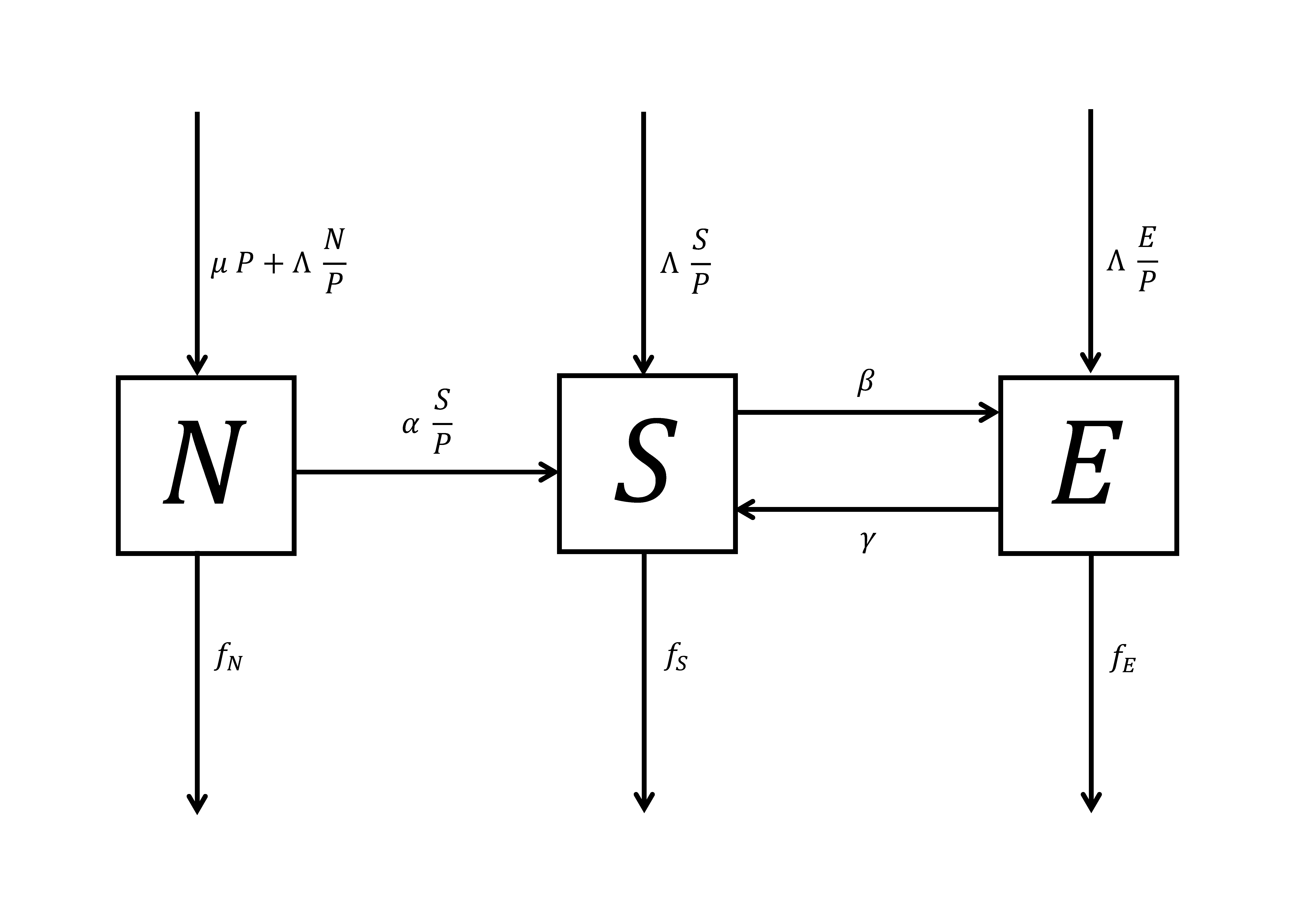
2.2. Flow diagram of smoking epidemic model
In this section, we discuss a flow diagram consisting of rectangular boxes and arrows which will represent each class and transitions between classes respectively.
Figure 1. Compartment model for population.
2.3. Model assumptions
We make the following assumptions for our model;
The parameter of a constant transition to time because the model of changes in smoking habits was only observed in a short period of time.
Everyone in a sub-population can interact with people in all other groups.
Transition between sub-populations \(S\) and \(E\) proportional to sub-population size.
However, the transition from \( N \) to \( S \) occurs because of the interaction and influence of smokers to non-smokers.
The death rate of a population that is independent on the density of each sub-population varies by \(d_n < d_e < d_s\).
The transition from \(E\) to \(S\) occurs because of the interaction between smokers and ex-smokers which results in the ex-smokers become smokers again.
2.4. Model representation
By taking the above assumptions into account and the transitions how people move among classes, we can construct a system of differential equations representing the model of the evolution of smoking behaviour as follows:
\begin{equation}\label{ode}\begin{cases}
\frac{dN}{dt} & = \mu P + \Lambda \frac{N}{P} – \alpha \frac{N S}{P} – (d_n +rP) N,\\
\frac{dS}{dt} & = \Lambda \frac{S}{P} + \alpha\ \frac{N S}{P} – \beta\ S + \gamma \frac{S}{P} E – (d_s +rP) S,\\
\frac{dE}{dt} & = \Lambda \frac{E}{P} + \beta S – \gamma \frac{S}{P} E – (d_e + r P)E.
\end{cases}
\end{equation}
(1)
It is noted that the total population is \( P = N + S + E \). From the above equation, we obtained:
\begin{eqnarray}
\frac{dP}{dt} & = & \frac{dN}{dt} + \frac{dS}{dt} + \frac{dE}{dt} \nonumber\\
& = & \Lambda + \mu\ P -(d_n + r P) N – (d_s + r P)S – (d_e + r P) E.
\end{eqnarray}
(2)
In order to have the same unit for every class, we scale the system equation (1) by dividing it with the total population \(N(t).\) This gives
\begin{equation}\label{odeproporsi}
\begin{cases}
\frac{ds}{dt}= \alpha s n + \gamma s e -(d_s-d_n)s-\beta s-\mu s +((d_s-d_n)s+(d_e-d_n)e)s,\\
\frac{de}{dt} = \beta s – \gamma s e -(d_e-d_n-\mu)e + ((d_s-d_n)s+(d_e-d_n)e)e,\\
\frac{dP}{dt} = \mu P + \Lambda -(d_n+rP+(d_s-d_n)s+(d_e-d_n)e),
\end{cases}
\end{equation}
(3)
where
\begin{equation}\label{Pers5}
s = \frac{S}{P}, \quad e = \frac{E}{P}\nonumber
\end{equation}
and
\begin{equation}\label{Pers6}
N = n \ P = \left(1 – s – e \right) P.\nonumber
\end{equation}
The domain of the System (3) is
\begin{equation}
\mathcal{D} = \left\{ \begin{bmatrix}
s\\
e\\
P
\end{bmatrix} \in \mathbb{R}^3 \ \Bigg\vert
\begin{array}{c}
s \geq 0,\\
e \geq 0,\\
s + e \leq 1,\\
P > 0.
\end{array} \right\}
\label{domain}.
\end{equation}
(4)
Theorem 1.
If the initial condition is located at \( \mathcal {D} \), then the system (3) with the initial condition has a single solution that exists and stays with \( \mathcal {D} \) for every time \( t \ge 0 \).
Proof.
The right segment of the system (3) is a continuous function with continuous partial derivatives at \( \mathcal {D} \), so the system (3) has a single solution. Next, note that if \( s = 0 \), then \( \frac {ds} {s} \ge 0 \) and if \( e = 0 \), then \( \frac {de} {s} \ge 0 \). If \( s + e = 1 \) then \( \frac {ds} {dt} + \frac {de} {dt} = – \mu 0 \).
If \( P> 0 \) for \( t = 0 \) then \( P > 0 \) for every \( t> 0 \), so that no orbit leaves \( \mathcal {D} \). As a result, there is a single solution for every time \( t \ge 0 \).
3. Equilibrium Points
There are two equilibrium points of the System (3): smoking-free and smoking-present equilibrium points.
3.1. Smoking-free Equilibrium point
The smoking-free equilibrium is the case where there is no smoker in the population. Therefore, the System (3) is evaluated for \( s = 0\). By setting \( \frac{ds}{dt} = 0, \frac{de}{dt} = 0, \frac{dP}{dt} = 0\) we get, \(s= e=0\) and \( P^* = \frac{\mu – d_n + \sqrt{(\mu-d_n)^2-4 \Lambda r}}{2r}\).
Thus, we can obtain the smoking-free equilibrium for the system of Equations (3)
\begin{eqnarray}
x_{dfe} =(0,0, P ^ *) \quad or \quad
x_{dfe} = \left(0,0,\frac{\mu – d_n + \sqrt{(\mu-d_n)^2-4 \Lambda r}}{2r}\right).\label{ekuilibrium}
\end{eqnarray}
(5)
By the next generation method, the reproductive number \(R_0\) for equilibrium point (5) is given below:
We refer Theorem 2 to use the reproductive number to analyse the stability of the smoke-free equilibrium (5).
Theorem 2.
Consider the system of (3) with the smoking-free equilibrium \( x_{dfe}\) given by (5) and the reproductive number \(R_0\) given by (6). If \(R_0 1\).
Based on the Theorem 2, we know that if the \(R_0 1\), then the smoking habit will invade the population.
3.2. Smoking-present equilibrium
In this section, we investigate the existence of the Smoking-present equilibrium for the reproductive number \(R_0 1\). For this purpose, we use the Newton-Raphson numerical method. The values of parameters are:
Table 1. Values of parameters.
Parameter
Value(\(year^{-1}\))
\(\mu\)
0.00162
\(\Lambda\)
180
\(d_n\)
0.00065
\(d_s\)
0.0013
\(d_e\)
0.000975
\(r\)
0.00000000065
\(\alpha\)
0.0381
\(\gamma\)
0.0325
\(\beta\)
0.0398
with initial condition \(s(0)= 0.4\), \(e(0)= 0.045\), and \(P(0)=2000000\).
The smoking-present equilibrium points is the solution of the system:
\begin{equation}\label{metodenumerik}
\begin{cases}
0 = & \alpha s n + \gamma s e -(d_s-d_n)s-\beta s-\mu s +((d_s-d_n)s+(d_e-d_n)e)s,\\
0 = & \beta s – \gamma s e -(d_e-d_n-\mu)e + ((d_s-d_n)s+(d_e-d_n)e)e,\\
0 = & \mu P + \Lambda -(d_n+rP+(d_s-d_n)s+(d_e-d_n)e)P.
\end{cases}\end{equation}
(7)
Based on the values of the parameters in Table 1, we get the reproductive numbers value that is \(0.67 < 1\). By the Newton-Raphson method, we get the solution (7) which is
\begin{equation}
x_{dfe}=[s,s_e,P]\nonumber
\end{equation}
where
We see that the point (8) is a smoking-free equilibrium point of (3). Therefore, we can say that the smoking-present equilibrium point for \(R_0 < 1\) does not exist.
Furthermore, it will be investigated the existence of the smoking-present equilibrium point for \(R_0 > 1\). Therefore, we choose the parameter \(\alpha = 0.0881\) and the other parameters as in Table 1, so that the reproductive number \(R_0 = 1.55 > 1.\) Therefore, the smoking-present equilibrium point for \(R_0 > 1\) is the solution of the system:
\begin{equation}\label{metodenumerik2}
\begin{cases}
0 = \alpha s n + \gamma s e -(d_s-d_n)s-\beta s-\mu s +((d_s-d_n)s+(d_e-d_n)e)s,\\
0 = \beta s – \gamma s e -(d_e-d_n-\mu)e + ((d_s-d_n)s+(d_e-d_n)e)e,\\
0 = \mu P + \Lambda -(d_n+rP+(d_s-d_n)s+(d_e-d_n)e)P.
\end{cases}\end{equation}
(9)
By the Newton-Raphson method, we get that the solution of system (7) is:
\begin{equation*}
x_{dfe}=[s,s_e,P]
\end{equation*}
where
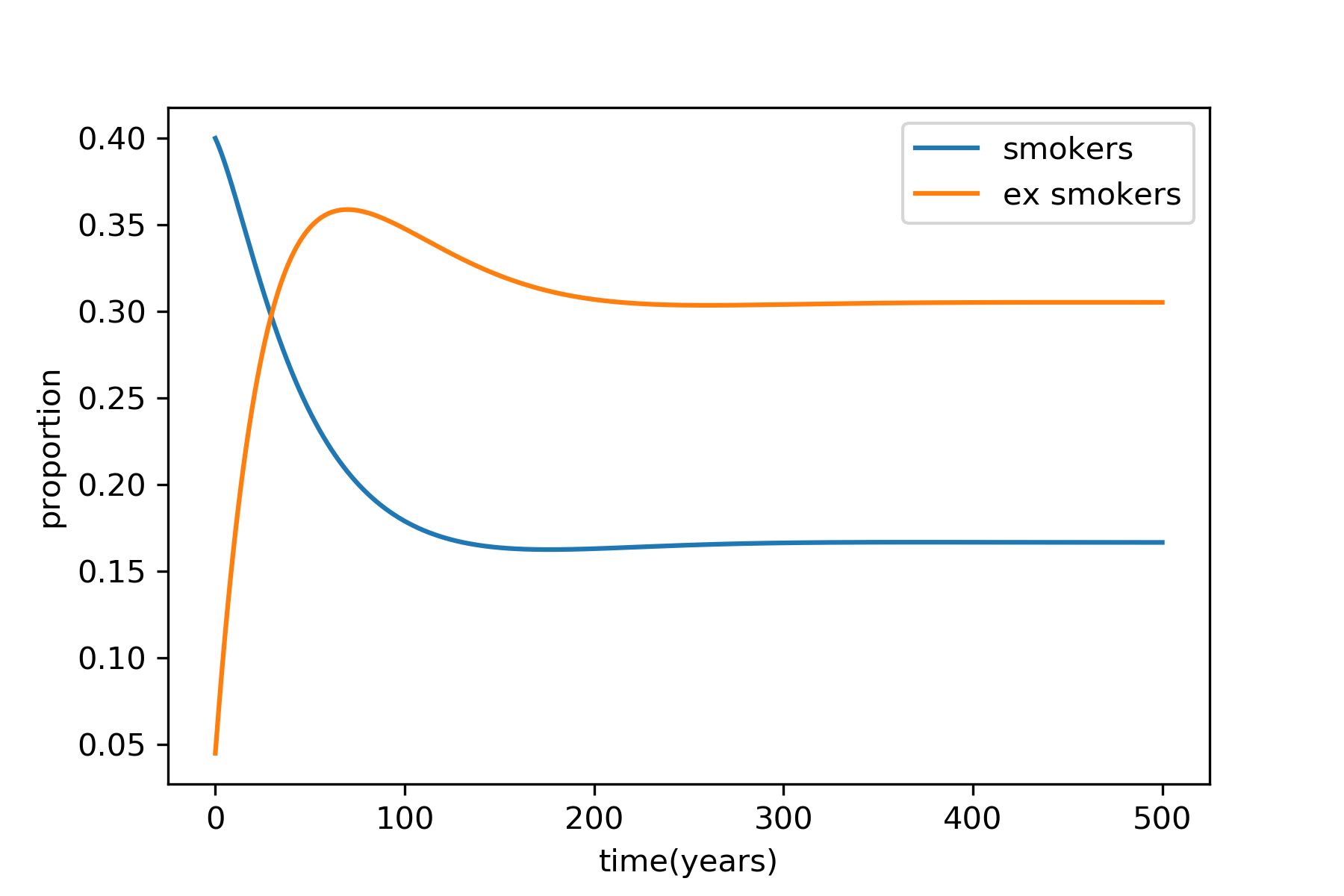
We see that the point (8) is a smoking-present equilibrium point of the System (3). Therefore, we can say that the smoking-present equilibrium point for \(R_0 > 1\) exist. This is reinforced by the illustration as follows:
Figure 2. The Smoker and Ex-Smoker Proportion vs Time for \(R_0 > 1\).
Based on the Figure 2, it is shown that both the smokers and the ex-smokers are stable at the smoking-present equilibrium point after \(300\)ss years.
3.3. Stability of the smoking-present equilibrium point
In this section, we will investigate whether the smoking-present equilibrium point is stable using the following definition numerically.
Definition 1. (Liapunov)
Let \( \bar{x}(t) \) be the solution of (3). A point \( \bar{x} (t) \) is called stable if, for every \( \epsilon> 0 \), there exists \( \delta = \delta (\epsilon)> 0 \) so that for any solution \( y(t) \) of (3) with \( | \bar{x}(t_0) -y(t_0) | < \delta \),
\[\begin{equation}
| \bar{x} (t) -y (t) | < \epsilon
\end{equation}\]
for all \( t> t_0\) and for all \(t_0 \in \mathbb{R} \).
There is also a concept of the asymptotic stability that is given below.
Definition 2. (Asymptotic stability)
A solution \(\bar{x} (t) \) is called asymptotically stable if \( \bar {x} (t) \) is stable and for every \(y (t)\) of the system of (3), there exists \(b>0 \) such that, if \( | \bar {x} (t_0) -y (t_0) | < b \) holds. Then
\begin{equation}
\lim_ {t \to \infty} | \bar {x} (t) -y (t) | = 0. \nonumber
\end{equation}
Based on this definition, an equilibrium point is said to be stable if a slight change in the initial value of the system will only result in a small change in the solution. For that, we put \(c=0.05\) and initial value
\(z_0=[s_0,e_0,P_0],\)
where
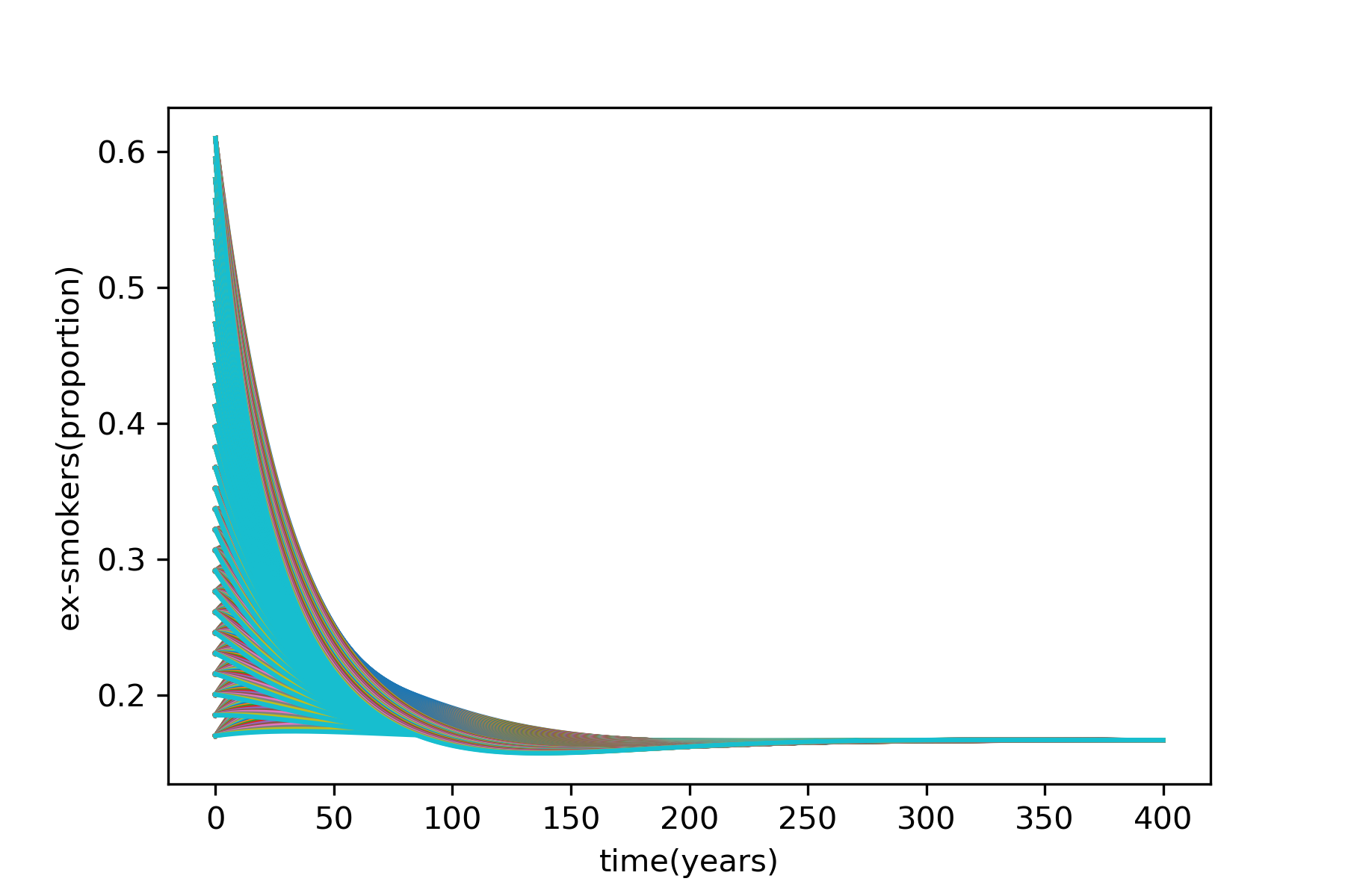
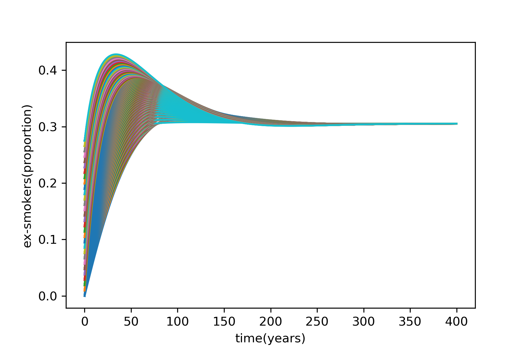
Based on the values of the parameters and the initial value \(z_0\), we get the result of numerical analysis of stability of the smoking-present equilibrium point (10) which is illustrated in the figure below:
Based on the Figure 3, We can see that for every initial value in (11), the solutions of the system will converge to the smoking-present equilibrium point. Therefore, we can conclude that the smoking-present equilibrium point of (3) is local asymptotically stable.
Figure 3. The Stability Analysis of Smoking Present Equilibrium.
4. Analysis of sensitivity parameters
Many doctors agree that smoking is bad for health, so the smokers need to be reduced for a healthy country. There are \(x\) methods to reduce the smokers population. First, prevent non-smokers from becoming smokers. Second, stop the smokers from their smoking habit. Third, prevent ex-smokers back to being smokers. Mathematically, there are \(3\) parameters which directly affect the smokers population: \(\alpha\), the rate of non-smokers become smokers; \(\beta\), the rate of smokers become ex-smokers; \(\gamma\), the rate of ex-smokers become smokers. In other words, if one of the parameters value is changed, it will alter the behaviour of smokers population in Indonesia. In consequence, in this section we will discuss
sensitivity of smokers class to parameters \(\alpha\), \(\beta\) and \(\gamma\) numerically. For that reason, the estimation chosen for the parameters \(\alpha, \beta\) and \(\gamma\) is \(0.0381 \leq \beta, \gamma,\alpha \leq 0.0681\).
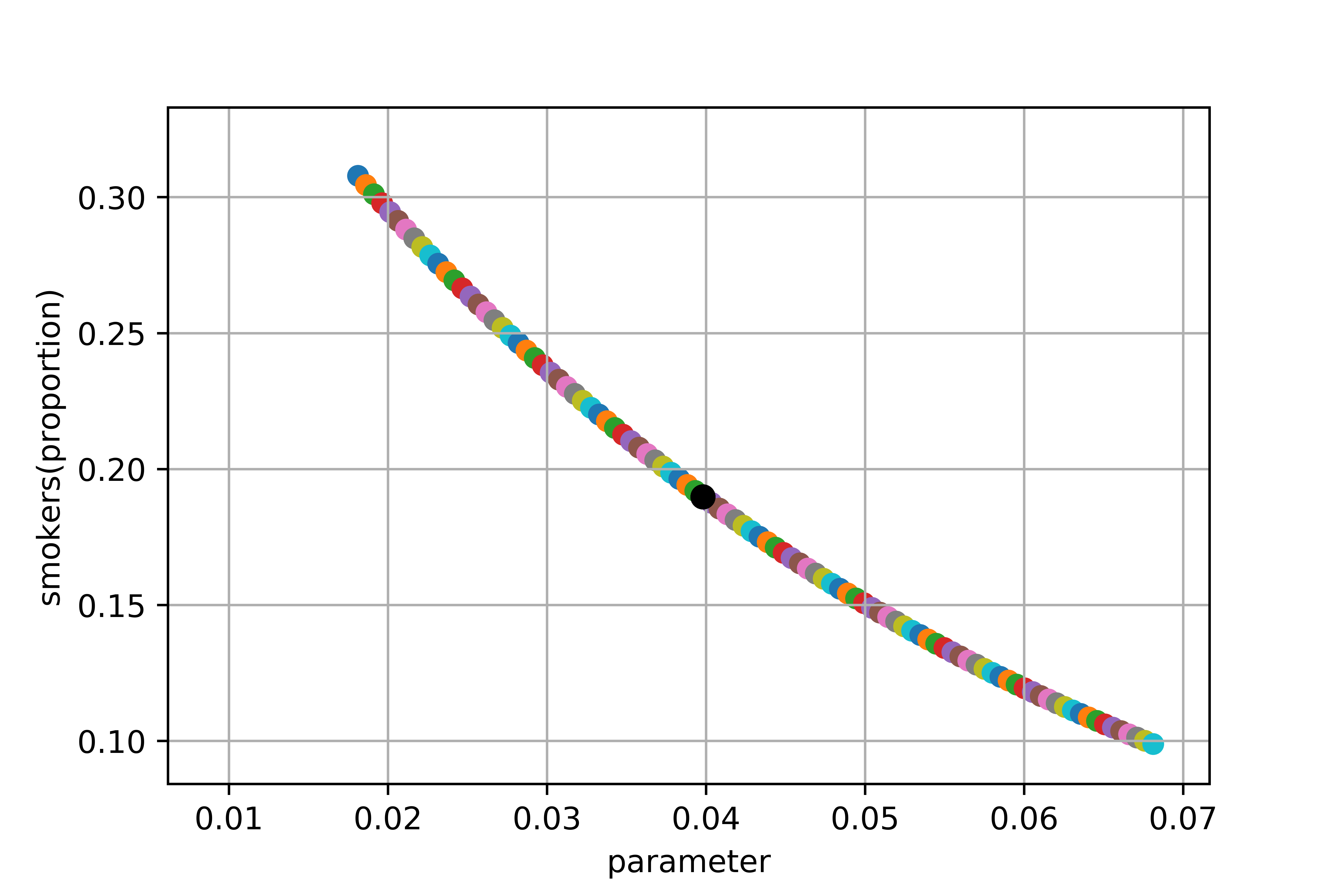
Figure 4. The Sensitivity Analysis of The Parameters \(\beta\).
In this Figure 4, we can see that the parameter \(\beta\) affects negatively the number of smokers.
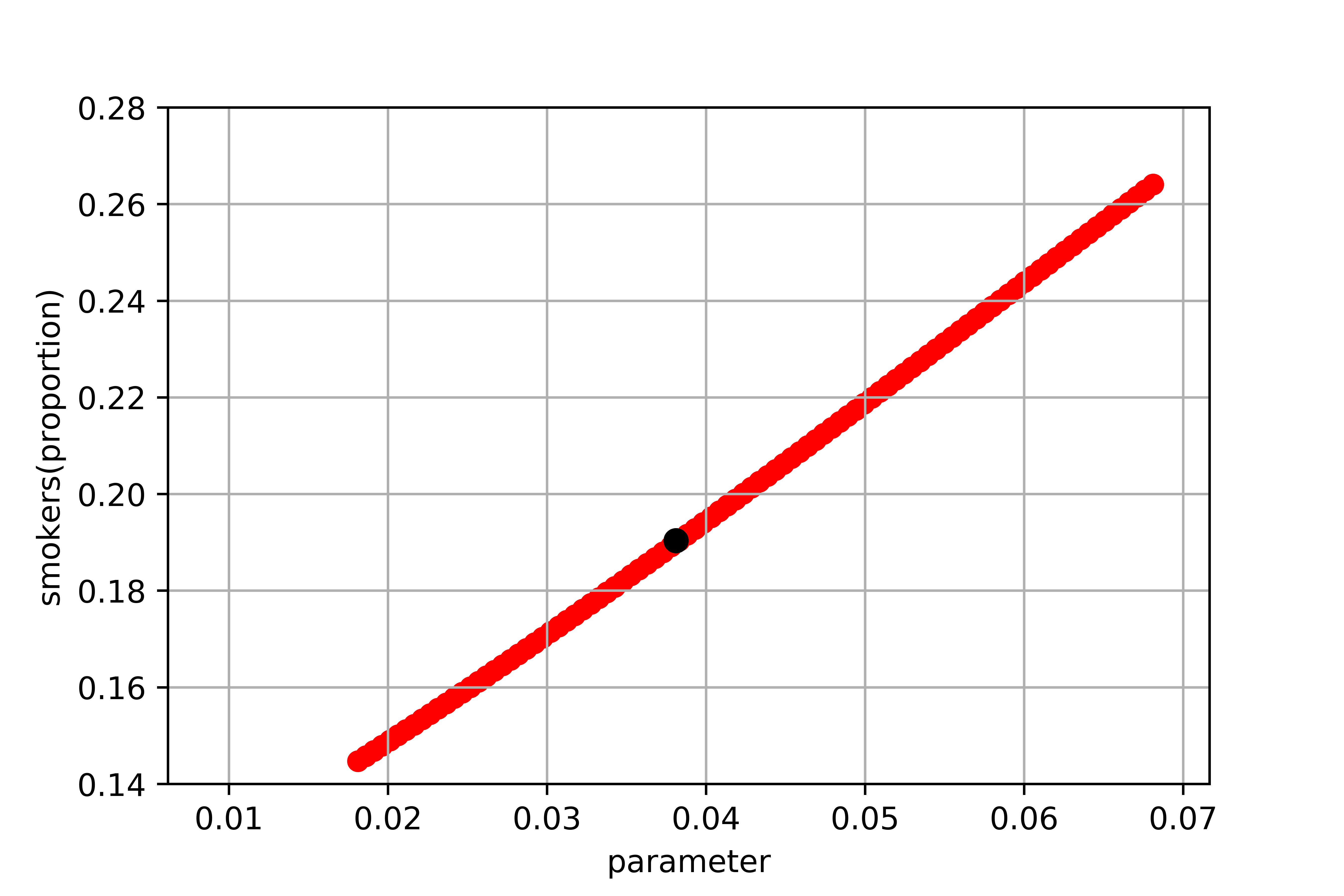
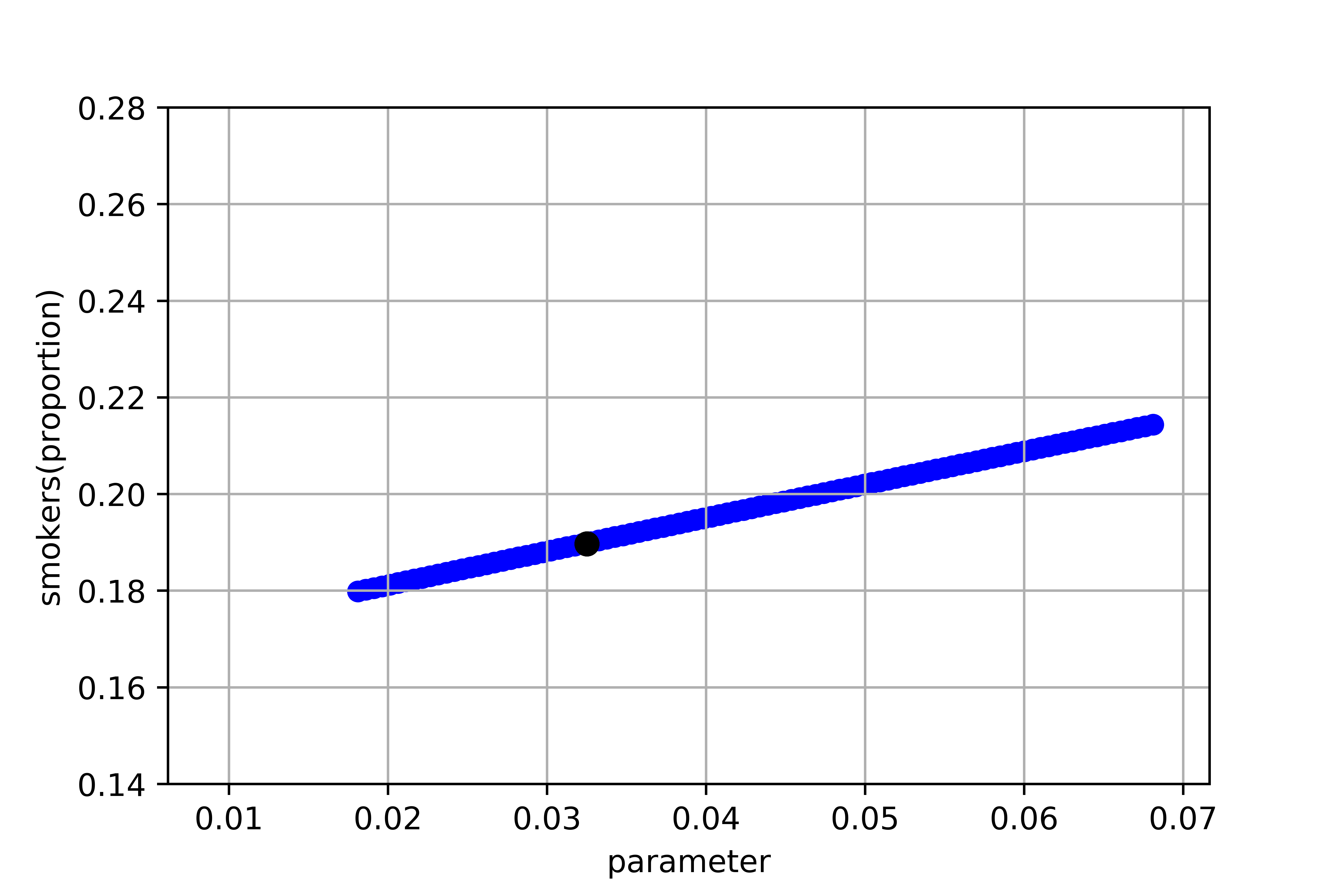
At the same time Figure 5 and Figure 6 shows that the increase of \(\alpha\) and the \(\gamma\) values leads to the increase of the number of smokers. The black dot in the Figure 4, Figure 5 and the Figure 6 indicates the value of the parameters \( \beta,\alpha \) and \(\gamma\) at time \(0\), which are \( 0.0398, 0.0325\) and \(0.0381\) respectively.
The above numerical results shows that the change of \(0.0005\) of the parameter \(\beta\) will change about \(0.0005\) of the proportion of the smokers \(s\).
Meanwhile, if the value of the parameters \(\alpha\) and \(\gamma\) change with increment \(0.0005\) then it will change of the number of smokers with increment \(0.0012\) and \(0.0003\) respectively.
In the end, we can say that the parameter \(\beta\) is the most sensitive for affecting the number of smokers.
Figure 5. The Sensitivity Analysis of The Parameters \(\alpha\). Figure 6. The Sensitivity Analysis of The Parameters \(\gamma\).
5. Conclusion
We have proposed a mathematical model for smoking behavior in Indonesia. There are two equilibrium points of the model that are smoking-free and smoking-present equilibrium points. We get that the smoke-free equilibrium point exists. Also, using the reproductive number, we get that the smoke-free equilibrium point is local asymptotically stable. At the same time, we get that the smoking-present equilibrium point exist. Also, by the numerical analysis we get that these point are local asymptotically stable. A numerical simulation using data in Indonesia has been done to see the behavior of smokers in Indonesia. We get that the smoker class is most sensitive to the rate of the smokers become ex-smokers. Furthermore, we can conclude that the best way to reduce the number of smokers in Indonesia is pushing the smokers to stop smoking.
Acknowledgments
The authors would like to express their thanks to the referees for their useful remarks and encouragements.
Author Contributions
All authors contributed equally to the writing of this paper. All authors read and approved the final manuscript.
Conflict of Interests
The authors declare no conflict of interest.
References
Castillo-Garsow, C., Jordan-Salivia, G., & Rodriguez-Herrera, A. (1997). Mathematical Models for the Dynamics of Tobacco Use, Recovery, and Relapse. Public Health, 84(4), 543–547.[Google Scholor]
Sharomi, O., & Gumel, A. B. (2008). Curtailing smoking dynamics: a mathematical modeling approach. Applied Mathematics and Computation, 195(2), 475-499.[Google Scholor]
Alkhudhari, Z., Al-Sheikh, S., & Al-Tuwairqi, S. (2014). Global dynamics of a mathematical model on smoking. ISRN Applied Mathematics, 2014, Article ID 847075, 7 pages.[Google Scholor]
Pang, L., Zhao, Z., Liu, S., & Zhang, X. (2015). A mathematical model approach for tobacco control in China. Applied Mathematics and Computation, 259, 497-509.[Google Scholor]
Hammadi, I. J. (2019). Analisis pada model matematika perubahan perilaku merokok dengan program python. (Doctoral dissertation, Universitas Gadjah Mada).[Google Scholor]
N. Chitnis and J.M Cushing and J.M Hyman. (2006). Coupled Fixed Point Theorem and Dislocated Quasi-Metric Space. Society for Industrial and Applied Mathematics, (67), 24–45.[Google Scholor]
Van den Driessche, P., & Watmough, J. (2002). Reproduction numbers and sub-threshold endemic equilibria for compartmental models of disease transmission. Mathematical Biosciences, 180(1-2), 29-48.[Google Scholor]
Wiggins, S. (1997). Introduction to applied nonlinear dynamical systems and chaos. Springer-Verlag Telos, ISBN: 0387970037,9780387970035.[Google Scholor]
BPPK. (2000). Buku Fakta Tembakau dan Permasalahannya di Indonesia. Kementerian Kesehatan Indonesia.[Google Scholor]
WHO. (2018). Indonesia Tobacco Factsheet 2018.
Guerrero, F., Santonja, F. J., & Villanueva, R. J. (2011). Analysing the Spanish smoke-free legislation of 2006: a new method to quantify its impact using a dynamic model. International Journal of Drug Policy, 22(4), 247-251.[Google Scholor]