
RBF is an important method for approximating and interpolating functions and solving differential equations (both ordinary and partial) for data with scattered node locations and in computation domain in higher dimensions as discussed in [1]. RBF methods were first introduced by [2], who was a geodesist at Iowa State University. In his proposed method, he simplified the computation of scattered data problem relative to the previously used polynomial interpolation. In many cases, RBF methods have been proved to be effective, where polynomial interpolation fails. RBF method are often used in topographical representation and other intricate \(3D\) shapes.
The use of RBF to interpolate scattered data problem emanated from the fact that the interpolation problem becomes insensitive to the dimension (\(d\)) of the space in which the data set lies. Recently, different RBF based methods have gained attention in scientific, computing and engineering applications such as functions interpolation [3, 4], numerical solutions to partial differential equation (PDEs) [5, 6, 7], Multivariate scattered data processing [8] and so on. The main advantages of this method are spectral convergence rates that can be achieved using infinitely smooth basis functions, geometrical flexibility and ease of implementation [9, 10].
The origin of RBFs can be traced back to [2], when Hardy introduced RBF multi-quadratics (MQ) to solve surface fitting on topography and irregular surfaces. As a field engineer from 1947 to 1951, Hardy was first interested in stream and ridge lines. Hardy believed that an interpolation method containing an exact fit of data to a topographical region should exist. After thorough investigation, he discovered what later become multiquadric (MQ). Prior to the knowledge of MQ, trigonometric and algebraic polynomials were employed. Due to the quadric surface, Hardy termed his method multiquadric. The MQ transformed scattered data to a very accurate fit model of graph or surface. Subsequently he considered the MQ as a consistent solution of biharmonic solution [10] to physically demonstrate its bravery. Other researchers like [11] extensively tested twenty-nine different algorithms on the typical benchmark function on interpolation problems and ranked the MQ-RBF and thin-plate splines TPS-RBF (introduced in [12] via employing the minimum bending energy theory of the surface of a thin plate) as top two candidates based on the following criteria: timing, storage, accuracy, visual pleasantness of the surface, and ease of implementation. Following the success recorded on researches, RBFs have become popular in the scientific computing world, such as computer graphics, data processing, and economics.
In 1986, Charles Micchelli developed the theory behind the MQ method, and proved that the MQ method matrix system is invertible [13]. Few years later, [14, 15] a collocating method was derived for solving partial differential equations using MQ. The breakthrough by Kansa triggered a research boom in RBF. The Kansa method is meshless and superior to the classical method due to some advantages such as: integration-free, ease of implementation and superior convergence. In addition, it may be of interest that even before Kansa’s pioneer work, Nardini and Brebbia (1983) [16] applied the function \(1+r\) without prior knowledge of RBFs as the basis function in the Dual Reciprocity Method (DRM) in the context of the boundary element methods (BEM) to get rid of domain integral effectively. Over the years, several researchers proposed different methods which include:
| \(n\) | Type of RBF | \(\varphi(r,\epsilon)\) |
|---|---|---|
| 1 | Gaussian | \(e^{-(\epsilon^{2}r^{2})} \) |
| 2 | Wedland | \( (1-\epsilon r)^{4}+(4r+1) \) |
| 3 | Thin Plate Spline (TPS) | \( r^{3}\log(r) \) |
| 4 | Multiquadric (MQ) | \(\left(1+\epsilon^2 r^2\right)^{\frac{1}{2}}\) |
| 5 | Inverse Multiquadric (IMQ) | \(\left(1+\epsilon^2 r^2\right)^{-\frac{1}{2}}\) |
RBF interpolation method use linear combinations of \(N\) (where \(N\) is the number of data sites), radial functions \(\varphi(r)\), where \(r=||x-x_{i}||\) and \(x_{i}\) are the centers in \(\mathbb{R}^{d}\), where \(d\) is the dimension of the problem. In this section, we are considering radial basis expansion to solve a scattered data interpolation problem in \(\mathbb{R}^{d}\). It is further assumed that
The coefficients \(a_{k}\) can be obtained by activating the interpolation conditions
Theorem 1. Let \(\varphi:=\mathbb{R}^{d}\longrightarrow\mathbb{R}\) be a strictly positive definite function on \( \mathbb{R} \). Then
Since we are considering basis functions that are strictly positive definite \((SPD)\): IMQ, Wedland and Gaussian, the Theorem 1 gives new bounds as seen in Equation (6).
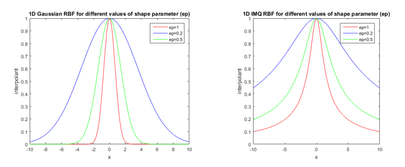
Note that \( \phi(\epsilon;r) =\phi(1;\epsilon ; r)\). If we take these radial basis as \( \phi(\epsilon;r)\), as a result, the bounds explain how \( \epsilon \) would behave on the shape of the function. i.e, increment in the value of \( \epsilon \) leads to a continuous alter of the shape of the function to a spiky shape as shown in Figure 1, where the spike is denoted by \(\phi(0)\). Conversely decrements in the value of an \( \epsilon \) leads to a continuous change in the shape of the function to a flat shape, having limit at \(\phi(0)\) as well, see Figure 1 for explanation.
Earlier in this section, we mentioned the role of the shape parameter (\(\epsilon\)). Several researchers worked in this direction [1, 22, 23, 24] but only few have discussed the role of shape parameter on the accuracy and shape of the interpolant. Numerous articles and books have been dedicated to explain how vital \(\epsilon\) is to determine the shape of a radial function therefore it is obvious that the shape parameter play a vital role in the accuracy and the shape of an interpolant, therefore, the shape parameter need to be chosen wisely.
The question is: how can we choose the optimal shape parameter \(\epsilon^{*}\) with least root mean square error (\(RMSE\))? The answer of this question will be discussed later in this section.
In an attempt to determine the interval in which the optimal shape parameter exists, different algorithms have been provided by different researchers but the purpose of this research work is to provide a Trial and Error algorithm. This algorithm explain explicitly the effect of shape parameter \( \epsilon \) on the the solution of PDE problems selected for interpolation and narrows the interval in which the optimal shape parameter \(\epsilon^{*}\) is obtain. This algorithm will be discussed in Subsection 3.2.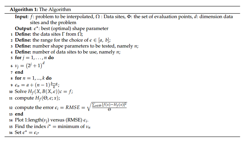
It can be observed that the lower values of \(\epsilon\) result in a \((flatter)\) basis function and the higher values of \(\epsilon\) result in a \((spikier)\) basis functions and \(\epsilon=0\) result to constant basis functions. Accuracy and stability are major concerns in numerical computations. It is well known that instability increases as \(\epsilon\) decreases. The significance of this statement lies in the fact that highest accuracy is often found at some small shape parameters, which may be in an unstable region. “Trade-off principle” is the term used to denote the conflict between accuracy and numerical stability [25]. The choice of the basis function is linked with this “trade-off principle”. Recently, different methods have been introduced to stably compute interpolants with small parameters by using an alternate basis, such as Contour-Pade and RBF-QR, as in [30] and [31].
Trial and Error Algorithm: To use Trial and Error algorithm, the PDE problems must be transform to matrix form i.e., \( Ab = f \), the generating data must be known [29]. If the function to be interpolate is unknown, it becomes very difficult to choose the best shape parameter. One of the easiest way to choose \((\epsilon^{*})\) is to perform a series of interpolation experiments on a large range of shape parameters then narrow it down to some selected shape parameters relative to least RMSE. Trial and Error algorithm enhances the clarification effectively on how shape parameter acts on solution of the PDE problems and gives an insight on how to narrow the interval of \( \epsilon \).
This scheme works only when the problem to be interpolated is known. We have the Algorithm 1:Example 1. Consider
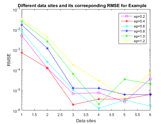
| \(N\) | \(\epsilon=0.2\) | \(\epsilon=0.4\) | \(\epsilon=0.6\) | \(\epsilon=0.8\) | \(\epsilon=1.0\) | \(\epsilon=1.2\) |
|---|---|---|---|---|---|---|
| 9 | 4.947883e-03 | 7.061068e-04 | 8.306327e-03 | 1.683301e-02 | 2.501740e-02 | 3.215444e-02 |
| 25 | 1.226119e-04 | 1.233554e-04 | 2.499596e-04 | 1.163722e-03 | 2.576520e-03 | 4.351338e-03 |
| 36 | 6.759435e-06 | 1.916602e-06 | 1.024839e-05 | 1.251879e-05 | 6.232077e-05 | 1.785228e-04 |
| 289 | 7.375946e-06 | 3.628324e-06 | 1.285584e-06 | 1.239982e-05 | 2.038053e-06 | 3.000325e-05 |
| 1089 | 2.659954e-06 | 1.588367e-06 | 3.208293e-06 | 6.096696e-06 | 3.424757e-05 | 4.013821e-06 |
| 4225 | 3.605753e-05 | 6.143375e-06 | 1.669543e-06 | 5.970569e-06 | 2.033888e-05 | 7.354744e-05 |

Example 2. Consider
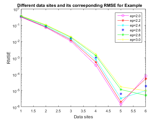
| \(N\) | \(\epsilon=1.0\) | \(\epsilon=1.2 \) | \(\epsilon=1.4\) | \(\epsilon=1.6\) | \(\epsilon=1.8\) | \(\epsilon=2.0\) |
|---|---|---|---|---|---|---|
| 9 | 5.361079e-02 | 6.657915e-02 | 7.686519e-02 | 8.599953e-02 | 9.281620e-02 | 9.719250e-02 |
| 25 | 7.972262e-03 | 1.192263e-02 | 1.633815e-02 | 2.100864e-02 | 2.578031e-02 | 3.055183e-02 |
| 36 | 2.857109e-04 | 6.473231e-04 | 1.210261e-03 | 1.977596e-03 | 2.933024e-03 | 4.050198e-03 |
| 289 | 1.659403e-06 | 4.254667e-06 | 9.665239e-06 | 2.699984e-05 | 5.940062e-05 | 1.145354e-04 |
| 1089 | 1.6725029e-06 | 3.219273e-06 | 1.395574e-05 | 1.838989e-06 | 1.024784e-06 | 4.224696e-07 |
| 4225 | 2.991273e-05 | 3.095514e-05 | 6.726647e-06 | 6.386367e-06 | 3.699115e-06 | 8.021659e-06 |

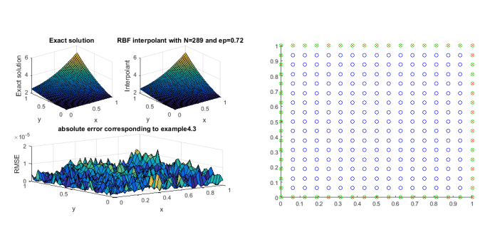
Example 3. Consider a second order PDE [32] \begin{equation*} \dfrac{\partial^{2}u}{\partial x\partial y}=4x+e^{x}, ~~~ (x,y)\in [0,1]\times[0,1] \end{equation*} with supplementary conditions \(\dfrac{\partial u(0,y)}{\partial y}= y,~~y\in[0,1], \) and \( u(x,0)= 2, ~~ x\in [0,1].\) The exact solution of this problem is \( u(x,y)=2x^{2}y+ye^{x}+\frac{y^{2}}{2}-y+2. \) Table 3 presents the RMSE for different data sites which correspond to Figure 6. The shape parameter that best fits the problem is tabulated in Table 6 and its corresponding figure is shown in Figure 7.
| \(N\) | \(\epsilon=0.70\) | \(\epsilon=0.72\) | \(\epsilon=0.74\) | \(\epsilon=0.76\) | \(\epsilon=0.78\) | \(\epsilon=0.80\) |
|---|---|---|---|---|---|---|
| 9 | 2.158636e+14 | 4.409283e+13 | 1.506239e+13 | 8.352088e+13 | 3.278437e+ | 5.099321e+ |
| 25 | 1.890692e+11 | 2.546641e+10 | 4.975475e+10 | 1.338177e+11 | 1.278434e+0014 | 1.367660e+11 |
| 36 | 9.573340e+02 | 1.349606e+04 | 8.731797e+03 | 1.758439e+04 | 1.274839e+04 | 6.150933e+04 |
| 289 | 1.606563e-05 | 1.632955e-05 | 7.146346e-05 | 4.759347e-06 | 6.556112e-05 | 2.439145e-05 |
| 1089 | 3.359890e-05 | 1.951918e-05 | 1.472573e-05 | 1.544620e-05 | 1.163340e-04 | 1.796294e-05 |
| 4225 | 3.174857e-05 | 3.725997e-05 | 2.397563e-04 | 2.986440e-05 | 3.321418e-05 | 1.772710e-04 |

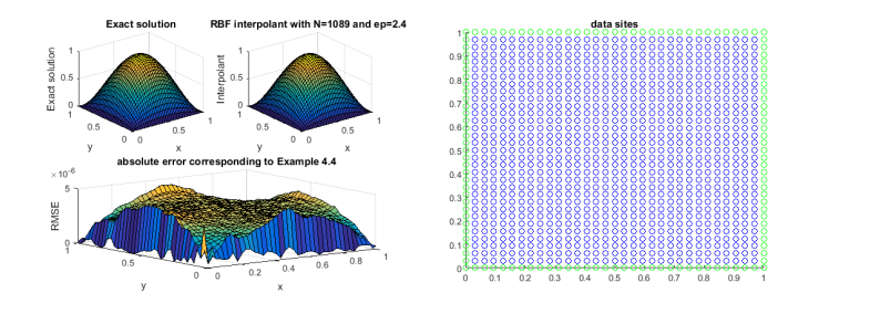
Example 4.
Consider PDE with variable coefficient: \begin{equation*} \begin{cases} (2-x^{2}-y^{2})\dfrac{\partial^{2}u}{\partial x^{2}}+\exp(x-y)\dfrac{\partial^{2}u}{\partial y^{2}}+2x\dfrac{\partial u}{\partial x}-\exp(x-y)\dfrac{\partial u}{\partial y}\\ =32y(1-y)(3x^{2}+y^{2}-x-2)-16x(1-x)(3-2y)\exp(x-y),~(x,y)\in[-1,1]^2 \end{cases} \end{equation*} with boundary conditions \(u(x,0)=u(x,1)=u(0,y)=u(1,y).\) The exact solution is \(u(x,y)=16x(1-x)y(1-y). \)
Table 4 presents the RMSE for different data sites which correspond to Figure 9. The shape parameter that best fits the problem is tabulated in Table 6 and its corresponding figure is shown in Figure 8.| Data sites | Example 1 \(\epsilon^{*}=0.4 \) | Example 2 \(\epsilon^{*}=1.6 \) | Example 3 \(\epsilon^{*}=0.72 \) | Example 4 \(\epsilon^{*}=2.4\) |
|---|---|---|---|---|
| 9 | 7.061068e-04 | 8.599953e-02 | 4.409283e+13 | 3.417120e-01 |
| 25 | 1.233554e-04 | 2.100864e-02 | 2.546641e+10 | 8.421439e-02 |
| 81 | 1.916602e-06 | 1.977596e-03 | 1.349606e+04 | 1.434081e-02 |
| 289 | 3.628324e-06 | 2.620360e-05 | 1.632955e-05 | 7.800962e-04 |
| 1089 | 1.588367e-06 | 2.699984e-06 | 1.951918e-05 | 3.327200e-06 |
| 4225 | 6.143375e-06 | 6.386367e-06 | 3.725997e-05 | 9.814452e-06 |

| Data sites | Example 1 \(\epsilon^{*}=0.4 \) | Example 2 \(\epsilon^{*}=1.6 \) | Example 3 \(\epsilon^{*}=0.72 \) | Example 4 \(\epsilon^{*}=2.4\) |
|---|---|---|---|---|
| 9 | 7.061068e-04 | 8.599953e-02 | 4.409283e+13 | 3.417120e-01 |
| 25 | 1.233554e-04 | 2.100864e-02 | 2.546641e+10 | 8.421439e-02 |
| 81 | 1.916602e-06 | 1.977596e-03 | 1.349606e+04 | 1.434081e-02 |
| 289 | 3.628324e-06 | 2.620360e-05 | 1.632955e-05 | 7.800962e-04 |
| 1089 | 1.588367e-06 | 2.699984e-06 | 1.951918e-05 | 3.327200e-06 |
| 4225 | 6.143375e-06 | 6.386367e-06 | 3.725997e-05 | 9.814452e-06 |