This paper considers the extension of the Adomian decomposition method (ADM) for solving nonlinear ordinary differential equations of constant coefficients to those equations with variable coefficients. The total derivatives of the nonlinear functions involved in the problem considered were derived in order to obtain the Adomian polynomials for the problems. Numerical experiments show that Adomian decomposition method can be extended as alternative way for finding numerical solutions to ordinary differential equations of variable coefficients. Furthermore, the method is easy with no assumption and it produces accurate results when compared with other methods in literature.
Differential equation can represent nearly all systems or phenomena undergoing change. They are quotidian in science, engineering and biology as well as in economics, social science, health and business [1]. Depending on the nature of the system at hand, differential equations may be linear, pseudo-linear or nonlinear. Often, systems described by differential equations are so complex, or the systems they represent are so large that a purely analytical treatment may not be tractable.
Many mathematicians have studied differential equations. A simple example is Newton’s second law of motion-the relationship between the displacement \(x\) and the time \(t\) of an object under the force \(F\) is given by the differential equation \[m\frac{d^{2}x(t)}{dt^{2}}=F(x(t)),\]
which constrains the motion of a particle of constant mass \(m\). In general, \(F\) is a function of the position \(x(t)\) of the particle at time \(t\).
Adomian decomposition method is a semi-analytical method for solving ordinary and partial nonlinear differential equations [2]. The method developed by George Adomian is also applied to solve both linear and nonlinear boundary value problems (BVPs) and integral equations. The numerical result is obtained with minimum amount of computation [3]. Adomian technique is based on a decomposition of a solution of nonlinear functional equation in a series of functions. Each term of the series is obtained from polynomial generated by a power series expansion of an analytic function [4]. Some of the advantages of the Adomian decomposition are; it can be applied directly for all types of functional equations both linear and nonlinear and it has ability of greatly reducing the size of computational work while still maintaining high accuracy of the numerical solution [4]. Adomian decomposition method (ADM) provides an analytical approximate solution for nonlinear functional equations in terms of a rapidly converging series without linearization, perturbation or discretization [5].
where \(L\) and \(N\) are linear and nonlinear operators respectively and \(f\) is a known function. By Adomian decomposition method, the solution \(u(x,t)\) of (1) is decomposed in the form of an infinite series
\begin{align}
&\label{8}
A_{n}(u_{0},u_{1},…,u_{n})=\sum^{n}_{k=1}c(k,n)N^{k}(u_{n}) \forall n\in N.
\end{align}
(8)
Wazwaz [8] suggested a new algorithm in which after separating \(A_{0}=N(u_{0})\) from other terms of the Taylor series expansion of the nonlinear function \(N(u)\), we collect all terms of the expansion obtained such that the sum of the subscripts of the components of \(u(x,t)\) in each term is the same.
Ibijola and Adegboyegun [9] considered the generalized first order nonlinear differential equation of the form
\begin{equation}
\label{9}
y’=f(t,y), y\in R^{d}, f : R X R^{1}\longrightarrow R^{1}
\end{equation}
(9)
with initial condition \(y(0)=y_{0}\in R^{d}\). In reviewing the basic methodology, an abstract system of differential equation
(9) assuming that \(f(t,y)\) is nonlinear and analytic near \(y=y_{0}\), \(t=0\) was considered. It is equivalent to solving the initial value problem (9) and the solution is obtained as
where \(\rho\) is a formal parameter. Functions \(A_{n}\) are polynomials in \(y_{1},y_{2},…,y_{n}\), which are referred to as the Adomian polynomials. The first few Adomian polynomials for \(d=1\) are listed by Zhu et al., [10] as:
where primes denote the partial derivatives with respect to \(y\).
It was shown by Himoun et al., [11] that the Adomian polynomials \(A_{n}\) are defined by the explicit formula:
where \(\sup_{t\in s}|f^{k}(t,y_{0})|\leq M\) for a given time interval \(j\subset R\).
Basically, there are two methods of generating Adomian’s polynomials using the orthogonality of functions \((e^{ln x},~n\in Z)\). The first method determines these polynomials explicitly whereas the second method generates them recursively. Different forms of nonlinearity are discussed in literature [13]. Cherruault and Adomian [14] suggested the following:
The assumption (16) is almost always satisfied in concrete physical problems. By (15) and (16), we have the form of Adomian series as a generalization of Taylor series:
Since \(\sum^{\infty}_{j=1}u_{j}(x,t)f^{j}(\rho)\) is absolutely convergent. By re-arrangement of terms in the right hand side of (20), we can write \(N(u_{\rho})\) as:
Many authors have used different forms of methods to solve (23) and (24) of constant coefficients. A few of these solution techniques are decomposition methods [15], differential transform method [16], double decomposition method [17], Taylor series method with numerical derivatives [18], homotopy perturbation method [19], projected differential transform method [20], generalized differential transform method [21], Picard iteration method [9] and Adomian decomposition method [7,22].
The main goal of this article is to extend the Adomian decomposition method by modification in order to obtain a polynomial solution of (23) and (24). Adomian decomposition method (ADM) solves nonlinear operator equations for any analytic nonlinearity providing an easily computable, readily verifiable and rapidly convergent sequence of analytic approximate solutions. Since it was first presented in the 1980’s, Adomian decomposition method has led to several modifications on the method made by various researchers in an attempt to improve the accuracy or expand the application of the original method [23]. The choice of decomposition is non-unique and provides a valuable advantage to the analyst, permitting the freedom to design modified recursion schemes for ease of computation in realistic systems [23].
In order to obtain the Adomian polynomial solution of (23) and (24), we write the nonlinear variable coefficient equation (23) in its operator form as:
where \(F\) is a known function and \(y\) is the unknown function to be determined, \(L\) is the linear operator to be inverted, \(R\) is the linear remainder operator and \(N\) is the nonlinear operator which is assumed to be analytic. We stressed that the choice for \(L\) and its pair \(L^{-1}\) (inverse of \(L\)) are determined by the equation being considered, hence the choice is non-unique. Here, we choose our \(L\) to be \(L=\frac{d}{dx}(.)\)
and thus its inverse \(L^{-1}\) follows as the one-fold definite integration operator from \(x_{0}\) to \(x\). Thus, we have \(L^{-1}Ly=y-\psi,\) which assumes the initial value \(\psi=y_{a}\).
For \(nth\)-order differential equation, the choice of \(L\) is \(L=\frac{d^{n}}{dx^{n}}(.)\) and its inverse \(L^{-1}\) is the \(n\)-fold definite integration operator from \(x_{0}\) to \(x\). Thus, \(\psi\) absorbs the initial value \(\psi=\sum^{n-1}_{k=0}\alpha_{k}\frac{(x-x_{0})^{k}}{k!}.\) Applying the inverse linear operator \(L^{-1}\) to both sides of Equation (25), we obtain
where the \(A_{k}’s\), which depend on \(y_{0}\),\(y_{1}\),…,\(y_{k}\) are called the Adomian polynomials and are obtained for the nonlinearity \(Ny=f(y)\) by
The first few Adomian polynomials for the one variable simple analytic nonlinearity \(Ny=f(y(x))\) have been listed by Zhu et al., [10] from \(A_{0}\) through \(A_{3}\), inclusively.
However, in this work, for equations with variable coefficients, we modified the above expressions for \(A_{0}\) through \(A_{4}\), inclusively, as
The \(y_{k}\)’s \((k=0,~1,~2,…,n)\) are then substituted into (27) to obtain the approximate solution.
2.1. Evaluation of the error
In this paper, error is defined as
\[\text{Error}=\max_{a\leq x\leq b}\left|\text{Exact Value}-\text{Approximate Value}\right|.\]
In case the exact solution is not available, the approximate solution is compared with those in literature.
2.2. Illustrative examples
The Adomian decomposition method (ADM) as extended and modified is demonstrated on some examples for first order nonlinear ordinary differential equations of variable coefficients. The results obtained are tabulated for comparison.
Example 1. Consider the first order nonlinear differential equation [24]:
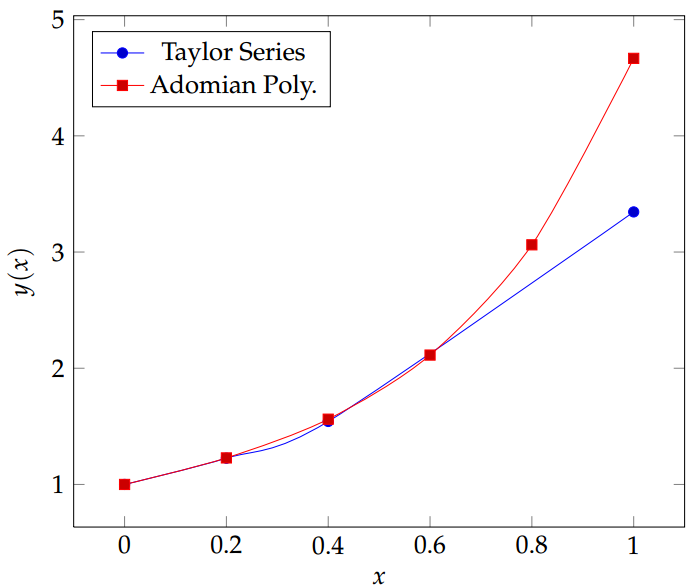
Table 1 shows that the solution by Taylor series method (TSM) and Adomian Decomposition method (ADM) are very close to each other at the points \(x=0.2\) and \(x=0.4\). Hyphens indicate that the function values are not available in literature.
Figure 1. The behaviour of the Taylor series method compared with the solutions using Adomian decomposition method (Example 1).
Figure 1 shows the behaviour of the Taylor series method compared with the solutions using Adomian decomposition method. Gap begins to exist between the two curves starting from the point \(x=0.6\).
Example 2. Consider the first order nonlinear differential equation [24]:
with the initial condition \(y(0.1)=1.\) The exact solution is \(y(x)=\frac{2}{2.01-x^{2}}\) and the solution by the Adomian Decomposition method is \(y(x)=0.98973+0.169367x-1.64583x^{2}+13.4375x^{3}-41.6667x^{4}+52.0833x^{5}\).
Table 2. Numerical results for Example 2.
x
Exact solution
Solution by ADM
Error
0.10
1.00000
1.00000
0.0000E-5
0.11
1.00105
1.00106
1.0000E-5
0.12
1.00220
1.00223
3.0000E-5
0.13
1.00346
1.00348
2.0000E-5
0.14
1.00482
1.00485
3.0000E-5
0.15
1.00629
1.00631
2.0000E-5
0.16
1.00786
1.00789
3.0000E-5
0.17
1.00954
1.00956
2.0000E-5
0.18
1.01133
1.01136
3.0000E-5
0.19
1.01322
1.01324
2.0000E-5
0.20
1.01523
1.01527
4.0000E-5
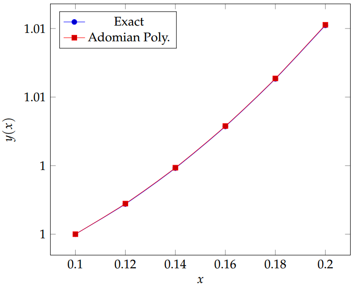
Figure 2. The behaviour of the exact solution and the approximate solution using Adomian decomposition method (Example 2).
Table 2 shows that the results by Adomian decomposition method (ADM) are very close to the exact values in terms of the absolute errors produced. Figure 2 shows the behaviour of the exact solution and the approximate solution using Adomian decomposition method. The curve by the Adomian decomposition method moves very close to the curve by the exact solution to the extent that gap between the two curves is not noticeable to the naked eyes.
Example 3. Consider the first order nonlinear ordinary differential equation [25]:
with the initial condition \(y(0)=1.\)
The solution by the Adomian decomposition method is \(y(x)=1+x+x^{2}+\frac{4}{3}x^{3}+\frac{5}{3}x^{4}+\frac{16}{15}x^{5}.\)
Table 3. Numerical results for Example 3.
x
Solution by TSMO(4)
Solution by ADM
0.0
–
1.00000
0.1
–
1.11151
0.2
1.25253
1.25367
0.3
–
1.44209
0.4
1.69318
1.69892
0.5
–
2.05417
0.6
–
2.54694
0.7
–
3.22677
0.8
–
4.15486
0.9
–
5.40536
1.0
–
7.06667
Table 3 shows that the solution by Taylor series method of order four (TSO(4)) produces results that are very close to the results produced by Adomian decomposition method (ADM) at the points \(x=0.2\) and \(x=0.4\). Hyphens indicate that the function values are not available in literature.
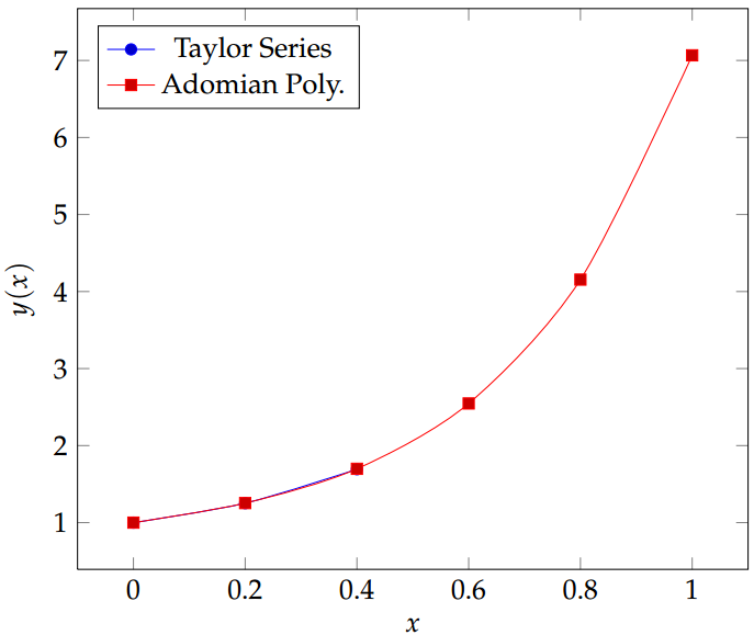
Figure 3. The behaviour of the Taylor series method of order four compared with the solutions using Adomian decomposition method (Example 3).
Figure 3 shows the behaviour of the Taylor series method of order four compared with the solutions using Adomian decomposition method. Only the two points available for the Taylor series method of order four are plotted (blue line). The two curves almost coincide with each other in the interval \((0.2,~0.4)\).
Example 4.
Consider the first order differential equation [24]:
with the initial condition \(y(1)=\frac{1}{\sqrt{2}}.\) The solution by the Adomian Decomposition method is \(y(x)=-1.34642+7.33484x-11.4929x^{2}+10.6446x^{3}-5.4401x^{4}+1.30000x^{5}\).
Table 4. Numerical results for Example 4.
x
Solution by MEM
Solution by ADM
1.0
1.00000
1.00000
1.1
–
1.11227
1.2
1.25478
1.25371
1.3
–
1.44140
1.4
1.69912
1.69808
1.5
–
2.05371
1.6
2.57034
2.54703
1.7
–
3.22713
1.8
4.27532
4.15499
1.9
–
5.40508
2.0
7.20134
7.06686
Table 4 shows that the modified Euler’s method (MEM) and Adomian decomposition method (ADM) produce results that are very close to one-another at the points \(x=1.0,~1.2,~1.4,~1.6,~1.8\) and \(2.0\). Hyphens indicate that the function values are not available in literature.
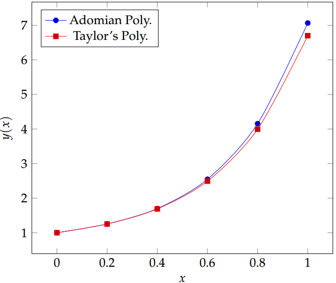
Figure 4. The behaviour of the modified Euler’s method compared with the solutions using Adomian decomposition method (Example 4).
Figure 4 shows the behaviour of the modified Euler’s method compared with the solutions using Adomian decomposition method. The two curves by the Adomian decomposition method and modified Euler’s method are very close to each other between the points \(x=0\) and \(x=0.4\). However, a noticeable gap starts to exist between them as from the point \(x=0.4\).
3. Discussion of results
The Adomian decomposition method (ADM) has been extended and discussed for the numerical solution of nonlinear ordinary differential equations of variable coefficients. The results obtained were compared with the exact solutions (where available) and some existing results in literature. The absolute errors obtained for example 2, as presented in Table 2 show that the results by the Adomian decomposition method (ADM) as extended are in excellent agreement with the exact solutions. Similarly, the results obtained compared well with those in literature as shown in Tables 1,3 and 4.
Author Contributions
All authors contributed equally to the writing of this paper. All authors read and approved the
final manuscript.
Conflicts of Interest
The authors declare no conflict of interest.
References
Abbasbandy, S., & Shivanian, E. (2009). Application of variational iteration method for nth-order integro-differential equations. Zeitschrift für Naturforschung A, 64(7-8), 439-444. [Google Scholor]
Wazwaz, A. M. (2000). A note on using Adomian decomposition method for solving boundary value problems. Foundations of Physics Letters, 13(5), 493-498. [Google Scholor]
Hosseini, M. M., & Nasabzadeh, H. (2007). Modified Adomian decomposition method for specific second order ordinary differential equations. Applied Mathematics and Computation, 186(1), 117-123. [Google Scholor]
Hosseini, M. M., & Nasabzadeh, H. (2006). On the convergence of Adomian decomposition method. Applied Mathematics and Computation, 182(1), 536-543. [Google Scholor]
Hasan, Y. Q., & Zhu, L. M. (2009). Solving singular boundary value problems of higher-order ordinary differential equations by modified Adomian decomposition method. Communications in Nonlinear Science and Numerical Simulation, 14(6), 2592-2596.[Google Scholor]
Cherruault, Y., & Adomian, G. (1993). Decomposition methods: a new proof of convergence. Mathematical and Computer Modelling, 18(12), 103-106. [Google Scholor]
Rach, R., & Baghdasarian, A. (1990). On approximate solution of a nonlinear differential equation. Applied Mathematics Letters, 3(3), 101-102. [Google Scholor]
Wazwaz, A. M. (2000). A note on using Adomian decomposition method for solving boundary value problems. Foundations of Physics Letters, 13(5), 493-498. [Google Scholor]
Ibijola, E. A., Adegboyegun, B. J., & Halid, O. Y. (2008). On Adomian Decomposition Method (ADM) for numerical solution of ordinary differential equations. Advances in Natural and Applied Sciences, 2(3), 165-170. [Google Scholor]
Zhu, Y., Chang, Q., & Wu, S. (2005). A new algorithm for calculating Adomian polynomials. Applied Mathematics and Computation, 169(1), 402-416.[Google Scholor]
Himoun, N. Abbaoui, K. & Cherruault, Y. (2003). Short new results on Adomian method. Kybernetes, 32, 523-539. [Google Scholor]
Abbaoui, K., & Cherruault, Y. (1995). New ideas for proving convergence of decomposition methods. Computers & Mathematics with Applications, 29(7), 103-108. [Google Scholor]
Abbaoui, K., & Cherruault, Y. (1994). Convergence of Adomian’s method applied to nonlinear equations. Mathematical and Computer Modelling, 20(9), 69-73.[Google Scholor]
Cherruault, Y., & Adomian, G. (1993). Decomposition methods: a new proof of convergence. Mathematical and Computer Modelling, 18(12), 103-106. [Google Scholor]
Bigi, D., & Riganti, R. (1986). Solutions of nonlinear boundary value problems by the decomposition method. Applied Mathematical Modelling, 10(1), 49-52. [Google Scholor]
Arikoglu, A. & Ozkol, I. (2007). Solution of fractional differential equations by using differential transform method. Computational Mathematics Applications, 41, 1237-1244.
Yang, Y. T., & Chien, S. K. (2008). A double decomposition method for solving the periodic base temperature in convective longitudinal fins. Energy Conversion and Management, 49(10), 2910-2916. [Google Scholor]
Miletics, E., & Molnárka, G. (2004). Taylor series method with numerical derivatives for initial value problems. Journal of Computational Methods in Sciences and Engineering, 4(1-2), 105-114. [Google Scholor]
He, J. H. (2003). Homotopy perturbation method: a new nonlinear analytical technique. Applied Mathematics and Computation, 135(1), 73-79. <a href="https://scholar.google.com/scholar?hl=en&as_sdt=0%2C5&q=Homotopy+perturbation+method%3A+a+new+nonlinear+analytical+technique.+[Google Scholor]
Jang, B. (2010). Solving linear and nonlinear initial value problems by the projected differential transform method. Computer Physics Communications, 181(5), 848-854. [Google Scholor]
Zou, L., Wang, Z., & Zong, Z. (2009). Generalized differential transform method to differential-difference equation. Physics Letters A, 373(45), 4142-4151. [Google Scholor]
Adomian, G. (1993). Solving Frontier Problems of Physics: The Decomposition Method. Springer, New York.
Duan, J. S., & Rach, R. (2011). A new modification of the Adomian decomposition method for solving boundary value problems for higher order nonlinear differential equations. Applied Mathematics and Computation, 218(8), 4090-4118. [Google Scholor]
Griffiths, D. F., & Higham, D. J. (2010). Numerical methods for ordinary differential equations: initial value problems. Springer Science & Business Media. [Google Scholor]
Jain, M. K., Iyengar, S. R. K. & Jain, R. K. (2012). Numerical Methods for Scientific and Engineering Computation (Sixth Edition). New Age International Publishers.