We calculate the electromagnetic field contained by a pulsed above a planar interface by using the modified Cagniard technique. The power density of spectrum of the wave that is observed at the distance from its emptily science usually differs from that of the source excitation, the power spectrum depends strangles on the speed of the wave in two media and the position of the observation point with respect to the interface and the source, form results of the rendition form a past source a discretely layer medium.
Keywords: Reflection, electromagnetic field.
1. Introduction
The Dipper effect which manifests itself when the source and the observer are in relative motion [1], when a pulsed wave propagates through an absorbing medium, the interplay of observer in accordance with the principle of consenting causes changes in the spectrum of the wave field [2] and mechanism is scattering by medium, the last two processes and their consequences for the wave field power density spectrum are described in [3,4, 5].
In this paper, we present the study of spectral changes, namely reflection at an interface. The discussion of the pulsed propagation in the two media configuration is carried out with the use of the modified Cagniard technique [6]. This method has bean successfully applied in electromagnetic [7, 8, 9, 10]. In this paper, we consider scalar waves fields. Explicit expressions for the system Green function are obtained and in this configuration the analysis of spectral changes can take place along the lies of the present paper as will. Furthermore, extended sources can be handled with the method as experienced in static dynamic problem as shown in [11].
2. Description of the configuration
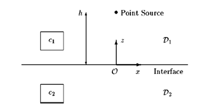
The two media configuration under consideration consist of the two and half space as shown in Figure 1. Orthogonal cartesian coordinates \((x,y,z)\) with respect to a fixed reference form are used. The reference frame is chosen such that the half-space and with \(z=0\), the point source is located with \(h\) as positive, the wave function speeds in two media are denoted by \(\varepsilon_{1}(z,\phi,0)\) and \(\varepsilon_{2}(z,\pi,0)\) respectively.
Figure 1.
The scalar wave is described by \(u=u(x,y,z,t)\) can be written as:
\begin{equation*}\label{eqn1}
u=u_0+\mathop{u}(1,z,\phi,0)\ \ \text{and}\ {\mathop{u}=\mathop{u}(2,z,\pi,0)}\,,
\end{equation*}
where \({\mathop{u}_{0}}\), is the wave function of the incident wave on the interface \(z=0\) and \({\mathop{u}_{1}}\) is the reflected wave in \(z,\ \phi,\ 0\) and \({\mathop{u}_{2}}\) is the transmitted wave field in \(z,\ \pi,\ 0\). The wave function satisfy the following wave equations:
\begin{eqnarray*}
(\nabla^2 – v_i^{-1}\frac{\partial}{\partial t}) \vec{u_i}(r,t)=-f(t)\delta(x,y,z-h)\ \ \ \ \text{for}\ \ \ z\geq 0\,,
\\\label{eqn3}
(\nabla^2 – v_i^{-1}\frac{\partial}{\partial t}) \vec{u_0}(r,t)=0\ \ \ \ \text{for}\ \ \ z=0\,.
\end{eqnarray*}
For \(t < 0 \), \(f(t)=0\) and \(u(r,t)=0\) and the boundary condition to be satisfied across the interface, we take
\begin{eqnarray*}\label{eqn4}
u_0+u_1=u_2,\ \ \text{at}\ z=0\ \ \ \ \text{for all}\ x,y\,,
\\\label{eqn5}
\frac{\partial}{\partial t}(u_0+u_1)=\frac{\partial}{\partial t}u_2,\ \ \text{at}\ z=0\ \ \ \ \text{for all}\ x,y\,.
\end{eqnarray*}
The electric field complex parallel in the interface in configuration of dielectric media, the incident wave field in the spectral wave
\begin{equation*}\label{eqn6}
\vec{u_0}(r,t)=\frac{f(t-R_0/C)}{4\pi R_0}\ \ \ \text{for}\ \ \ R_{0} \geq 0\,,
\end{equation*}
where
\begin{equation*}\label{eqn7}
R_0=[x^{2} +y^{2} +(z-h)^{2} ]^{\frac{1}{2} }\,.
\end{equation*}
The one-side usual Laplace transform with respect to \(t\) is:
\begin{eqnarray*}\label{eqn8}
E(x,s)=\int _{-\infty }^{\infty }\exp (-s\tau ) E(x,\tau )d\tau
\\\label{eqn9}
\vec{u}_0(s)=\frac{f(s)}{4\pi R_0}\exp^{-sR_0/v}\ \ \ \text{for}\ \ R_0 \geq 0\,.
\end{eqnarray*}
The reflection problem will be solved with the aid of the modified Cagniard method. The wave function to one sided Laplace transform with transform
\begin{equation*}\label{eqn10}
E(x,s)=\int _{-\infty }^{\infty }\exp (-s\tau ) E(x,\tau )d\tau\,.
\end{equation*}
The special Fourier transform for the representation of \(u(x,y,z,t)\) in the coordinates \(x\) and \(y\) parallel to the interface, scattered by a fields of \(s\) is given as:
Note: \(R\) and \(T\) remain bounded for all real values of the parameter \(\alpha\) and \(\beta\). Substituting Equations (2), (3) and (4) into Equation (1) tends to the representation of \(u, s\) and taking into account the algebraic factors of \(s\) and \(f(s)\) in the expression (2) – (4), we aim the representation
The system Green function \(g\) can be written into the form
\begin{equation*}\label{eqn22}
g(x,y,z,s)=\int_{-\infty }^{\infty }\exp (-s\tau ) g(x,y,z,\tau )d\tau
\end{equation*}
where \(T\) is a real variable of integration. The Laplace transformation in the time domain equivalent to the equation (5):
\begin{equation*}\label{eqn23}
u(x,y,z,t)=\frac{\partial }{\partial t} \int_{\tau }^{t}f(t-\tau ) g(x,y,z,\tau)d\tau
\end{equation*}
for \(\tau \leq t\leq \infty\) and equal to \(0\) for \(-\infty \leq t\leq \tau\) such that
\begin{eqnarray*}\label{eqn24}
\tau =i(\alpha x+\beta y)+\gamma_{1} (z+h)\ \ \text{for reflected wave}
\\\label{eqn25}
\tau =i(\alpha x+\beta y)+(\gamma_{1}h – z\gamma_2)\ \ \text{for transmitted wave}
\end{eqnarray*}
\(\alpha\) and \(\beta\) are replaced by \(p, q\) as:
\begin{equation*}\label{eqn26}
\alpha =p\cos \theta +q\sin \theta i,\ \ \beta =p\sin \theta -q\cos \theta
\end{equation*}
where \(x=r\cos \theta,\ \ y=r\sin \theta\) with \(0\leq r\leq \infty,\ 0\leq \theta \leq 2 \pi\) under then transformation \(\alpha^{2} +\beta^{2} =p^{2} +q^{2}\) and \(d\alpha d\beta =dpdq\) while
\begin{equation*}\label{eqn27}
u(r,s)=\frac{s^{2}}{4\pi i}\int dq \int_{-\infty }^{\infty }\exp (-iprs) u(p,q,z,s)dp\,.
\end{equation*}
Furthermore,
\begin{eqnarray*}\label{eqn28}
\gamma_{1,2}(p,q)=[\varphi_{1,2}(q,-p)]^{\frac{1}{2}}\ \ \text{with},
\\\label{eqn29}
\gamma_{1,2}^{-2}(p,q)+q^{2} = [\varphi_{1,2}(q,-p)]^{2}\ \phi, 0\,.
\end{eqnarray*}
The integral with respect to \(p\) is contained analytically into the contour of complex plane — under the application of Cauchy theorem. We will obtained to spec trial of the reflected wave in its dependence
\begin{equation*}\label{eqn30}
u(r,s)=\frac{s^{2}}{4\pi i}\int _{-\infty }^{\infty}dq \int_{-i\infty }^{+i\infty }\exp (-ipr+-s\gamma h_{1})(z+h)\frac{R(p,q)}{2{\mathop{\gamma }_{1}}(p,q)}dp\,.
\end{equation*}
We deform the path of integration into the modified Cagniard path
\begin{equation*}\label{eqn31}
pr+\gamma_{1} (h+z)=\tau\,,
\end{equation*}
with \(t\) real and positive. For a fixed value of \(\tau\), we have either two complex conjugate solution of \(p\) two are given
\begin{equation*}\label{eqn32}
p_{1} =\frac{r}{r^{2}+(z+h)^{2}} \tau +i\frac{(z+h)}{r^{2} +(z+h)^{2}}[\tau ^{2} -T_{1} (q)]^{\frac{1}{2}}\,,
\end{equation*}
for \(T_{1} (q)\leq \tau \leq \infty\) with \(T_{1} (q)=\{ r^{2} +(z+h)^{2} \varphi (q)\}\). Then
\begin{equation*}\label{eqn33}
u(r,s)=\frac{s^{2} }{4\pi i} \int_{-\infty }^{\infty }dq \int_{-i\infty}^{+i\infty }\exp (-s\tau i){\mathop{j}_{m}} Im\frac{R(p,q)}{2{\mathop{\gamma }_{1}} (p,q)} \frac{\partial {\mathop{p}_{1}}}{\partial \tau} d\tau\,.
\end{equation*}
The transpose green function follows as:
\begin{equation*}\label{eqn34}
g(r,\tau )=\frac{1}{\pi ^{2}} \int_{0}^{\tau}Im \frac{R(p,q)}{2{\mathop{\gamma}_{1}} (p,q)} \frac{\partial {\mathop{p}\nolimits_{1}}}{\partial \tau} dq\,,
\end{equation*}
with \(T(0)\leq \tau \leq \infty\) and equal to \(0\) for \(-\infty \leq \tau \leq {\mathop{T}_{1}} (0)\).
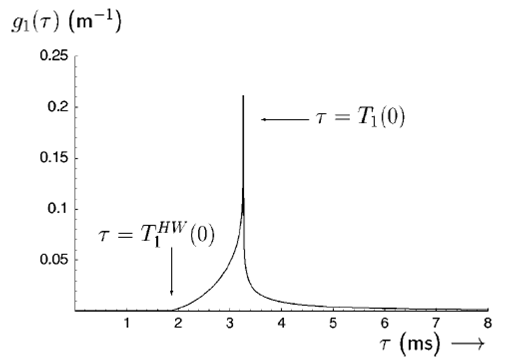
Figure 2.
The calculation of the Green function for this case is obtained according to the last equation in the representation of \(g(x,y,z,t)\), takes break points in term as first make the arrival lies of the head wave and the second less only a body wave contribution occurs.
3. Numerical results
The numerical integration and time conversation resulting from the modified Cagniard method wave carried out with the half of the Green function. We first note that the on–cases Green function for the reflected field is now given by
\begin{equation*}\label{eqn35}
g(0,z,t,\tau )=\frac{1}{4\pi} \frac{R(t)}{z+h}
\end{equation*}
with \(T(0)\leq \tau \leq \infty\) and equal to \(0\) for \(-\infty \leq \tau \leq T_{1} (0)\).
Green function \(G(T)\) for the case \(c1=330\) m/s, \(c2= 150\) m/s the source is at \(z=0,1\) and \(r=0\). Observation point is at \(r=1 m,\ z=0,1 m\) such that this case hand –wave arrival lies at \(T(0)=1.8\) ms and body–wave arrival time \(T(0)=3.3\) ms. In the previous has \(c1\) is largest from \(c1\), upon intersection the two wave speeds head may accordingly can be the case the Green function \(g(T0)\) is given in Figure 2.
4. Conclusion
We calculate the electromagnetic field by a pulsed point source above planar surface, the observed power spectrum depended strongly on the wave speeds, it the two media and on the positive of the observation point with respect to the interface and the source.
Acknowledgments
The author would like to express his thanks to the referee for useful remarks.
Author Contributions
All authors contributed equally to the writing of this paper. All authors read and approved the final manuscript.
Conflict of Interests
The author declares no conflict of interest.
References
Van Bladel, J. (1984). Relativity and engineering, Springer Berlin sec. in particular Chapter 15.[Google Scholor]
Oughstun, K. E., and Shenon, G. C. (1947). Electomagnetic pluse propagation in central Dielectric, springer, Berlin.
Wait J. R. (1986). Electromagnetic waves theory, State place New York, Wiley. Chapter 5.
Hill, D. A., & Wait, J. R. (1981). HF ground wave propagation over mixed land, sea, and sea-ice paths. IEEE Transactions on Geoscience and Remote Sensing, (4), 210-216.[Google Scholor]
Cagniard, L. (1939). Reflection and refraction of progressive seismic waves (p. Vii). Paris: Gauthier-Villars.[Google Scholor]
Kuester, E. (1984). The transient electromagnetic field of a pulsed line source located above a dispersively reflecting surface. IEEE transactions on antennas and propagation, 32(11), 1154-1162.[Google Scholor]
Abo-Seliem, A. A. (1998). The transient response above an evaporation duct. Journal of Physics D: Applied Physics, 31(21), 3046.[Google Scholor]
Doak, P. E. (1952). The reflexion of a spherical acoustic pulse by an absorbent infinite plane and related problems. Proceedings of the Royal Society of London. Series A. Mathematical and Physical Sciences, 215(1121), 233-254.[Google Scholor]
Widdet, D.V. (1946). The Laplace transform, Prinleton university press prinecton NJ.[Google Scholor]
Mandel, L., & Wolf, E. (1995). Optical coherence and quantum optics. Cambridge university press.[Google Scholor]
I.H.M.T. Van der Hijdem. (1987). Propagation of Transmition electric wave in stratfield, Anisctropic Media (North — Holand), Amsterdam.