In this paper, we examine linear and nonlinear boundary sinks in compartments whose adjacent sides are separated with sieve partitions allowing transport of chemical species. The sieve partitions serve as boundary sinks of the system separating each compartment from the subsequent one. With assumption of unidirectional transport of chemical species, constant physical properties and same equilibrium constant, system of partial differential equations are derived. The spatial variables of the derived PDEs are discretized using Method of Lines (MOL) technique. The semi-discrete system formed from this technique produced a system of 105 ODEs which are solved using MATLAB solver ode15s. The results show that for strongly nonlinear boundary sinks, concentration profile maintains low profile in interconnected adjacent compartments. This suggests that as nonlinearity increases at the boundary, the concentration profile becomes increasingly low in subsequent compartments.
Boundaries are integral parts of chemical reactor systems. Reactions taking place there often need to be carefully accounted for whenever meaningful designs leading to optimum yield of products are required. The type of reaction taking place at such boundaries may have unwanted significant effect on the concentration profile of any species of chemical being transported through such systems.
Several models exist in literature, while some are lumped parameter models [1,2,3], others are distributed parameter systems [4,5,6,7,8,9,10]. Some researchers [11] emphasized difficulty in obtaining the desired concentration profile if only inlet concentrations are dependent on. They investigated chemical reaction scheme involving favourable kinetics as can be found in the work of Lu et al., [12], but their work did not include diffusion of reacting species as the focus was on distributed source using a set of hyperbolic partial differential equations for an isothermal tubular reactor. Hamel et al., [13] investigated parallel series reactions in a one-dimensional, isothermal, isobaric tubular reactor. However, their work centred on lumped parameter system which was based on systems of Ordinary Differential Equations (ODEs) hence spatial effects on the reactants were not considered.
Nocon [14] on the other hand modelled distributed feed in continuous sedimentation where he presented a distributed source model in comparison with the standard point source model using a proposed distribution function, but the work included settling velocity which may not be required in systems where sedimentation is not considered. Some other researchers [15] modelled the effects of numbers and locations of inlet apertures on the flow field but their work centred on single-compartment system with emphasis on flow pattern and pictorial representation of the flow field.
Investigation was made by Adedire and Ndam [16] to model chlorine decay through water and intermediate Pseudomonas aeruginosa in multiple-compartment isothermal reactor, their research centred mainly on linear boundary sinks across the interconnected systems. Also, in their work [17], the focus was on comparison of species transport through the single and the interconnected multiple-compartment systems. They did not consider probable effects of nonlinear boundary sinks. They also did not investigate whether such nonlinearity has any significant effect on the concentration profiles in adjacent compartments for the species being transported through the interconnected systems.
Motivation to proceed on this study stems from process industries with continuous flow reactors consisting of chemical species with linear chemical sinks passing through material sieves such as aluminium or zinc sieve partitions acting as linear/nonlinear boundary sinks in interconnected multiple-compartment systems. It should be noted that the materials of the sieve partitions or any material attached to it will – to some extent – determine whether linear or nonlinear chemical sinks are taking place at the boundaries of each compartment as the chemical species moves through it. While the effects of wall decay in distribution systems have been considered in single-compartment systems, satisfactory investigation into linear/nonlinear boundary sinks of interconnected multiple-compartment systems with sieve or permeable partitions has not been done in an elaborate way.
To this end, this research intends to determine whether nonlinear boundary sinks will significantly alter the concentration profiles of adjacent compartments than linear boundary sinks of interconnected multiple-compartment isothermal systems. Do we need to consider species transport through the interconnected multiple-compartment systems for chemical species with nonlinear boundary sinks the same way as for linear boundary sinks? It should be noted that while some similar researches in literature use differential equations with either reactions terms only or diffusion-reaction terms only [5,6], this research use convection-diffusion-reaction terms with emphasis on PDEs that are incompletely parabolic whose details can be found in [18].
In this study, we examine linear and nonlinear boundary sinks for interconnected multiple-compartment isothermal systems with sieve partitions in order to determine the extent of linear/nonlinear boundary effects on the concentration profiles in adjacent compartments for species being transported through multiple-compartment system.
The remaining part of this paper is organized as follows: Section 2 centres on model development. Section 3 deals with numerical simulation of the derived model equations. While in Section 4, the results of the model simulation are presented with discussion. Conclusion comes up in Section 5.
2. Model development
The governing partial differential equations are developed from the concept that fluid is a continuum [19]. Define a function \(\Psi (\mathop x\limits^\_ ,t):\mathbb{R}^n \times \mathbb{R} \to \mathbb{R}\), where \(\Psi (\mathop x\limits^\_ ,t)\) is the concentration of species \(\xi \) flowing in n-dimensional space with variables \(\mathop x\limits^\_ \in \mathbb{R}{}^n\) such that \(\overline x = x_1 ,x_2 ,…x_n \) and t is time.
Figure 1. Schematic representation of species transport with linear/nonlinear boundary sinks through interconnected multiple-compartment isothermal system.
For \(n=1,\) we set up mass balance with assumption of convection and diffusion taking place along \(x_1\)-axis for the chemical species \(\xi \) with flux \(q_\xi \) and reaction term \(R_\xi \) over the infinitesimal thickness \(\Delta x_1 \) in the \(x_1 \) –direction of each compartment of the chemical reactor as
Let \(Q \subset \mathbb{N}\) be a finite set and \(\gamma \in Q\) , define \(Q = \left\{ {1,2,…,m} \right\}\) such that the least upper bound and greatest lower bound of Q are contained in Q, consequently Q is a bounded set.
Given the \(\gamma^{th} \)-compartment, if \( {\gamma } = 1,2,…m \in Q \subset \mathbb{N}\) for any m-compartment system, then the governing model Equation (4) becomes a system of m PDEs
Observe that (5), (6) and (7) are valid equations only in the specified domain of any \(\gamma^{th} \) compartment for each of the PDEs.
Since Equations (5), (6) and (7) for \(m-\)compartment system have first order derivatives in time and second order derivatives in space, their auxiliary conditions will include one initial condition and two boundary conditions in each \(\gamma ^{th} \) compartment of the system. Thus, for interconnected boundary conditions linking the state of concentrations in \((\gamma + 1)^{th} \) compartment with that of the preceding \(\gamma^{th} \) compartment, each \(\gamma^{th} \) compartment of the m-compartment system (5)-(7) will have the following initial and Dirichlet boundary conditions:
where \(\beta \in \mathbb{R}\) for some equilibrium constant k. Observe that the boundary condition given in (10) is interconnected boundary condition linking concentrations in the \(({\gamma} + 1)^{th} \) compartment with that of the preceding \({\gamma}^{th} \) compartment in a way showing the relationship at the boundary.
For m-compartment system showing continuity of flux of species \(\xi \) from \(({\gamma} – 1)^{th} \) compartment to \(\gamma^{th} \) compartment, the following initial and boundary conditions hold
The terms of (14), (18), (22), (26) and (30) from the left hand side denote net accumulation, convection, diffusion and first order reaction kinetics.
Each of the boundary conditions (17), (21), (25), (29) and (33) links the action in one compartment to the preceding compartment via linear/nonlinear sinks. Observe that there are linear/nonlinear sinks which act as nexus between the boundaries. Equations (20), (24), (28) and (32) show the continuous flux of the chemical species from one compartment to another.
2.1. Existence and uniqueness of solution
In this subsection, we present the existence and uniqueness of solutions for the system of PDEs and auxiliary conditions (14)-(33). Let \(\overline x = (x_1 ,…,x_n )\) , \({0}\le x_i < \infty ,\) \(1 \le i \le n\), be space variables and consider the system of PDEs
\begin{equation}
\label{e34}
\left. {\begin{array}{*{20}c}
{\psi _t (\overline x ,t)_1 = \sum\limits_{\left| v \right| \leqslant m}^{} {\left[ {A_v (\overline x ,t,\psi (\overline x ,t)_1 )\frac{{\partial ^{\left| v \right|} }}
{{\partial x_1^{v_1 } …\partial x_s^{v_s } }}} \right]\psi (\overline x ,t)_1 + G(\overline x ,t)_1 } } \\
{\psi _t (\overline x ,t)_2 = \sum\limits_{\left| v \right| \leqslant m}^{} {\left[ {A_v (\overline x ,t,\psi (\overline x ,t)_2 )\frac{{\partial ^{\left| v \right|} }}
{{\partial x_1^{v_1 } …\partial x_s^{v_s } }}} \right]\psi (\overline x ,t)_2 + G(\overline x ,t)_2 } } \\
. \\
. \\
. \\
{\psi _t (\overline x ,t)_s = \sum\limits_{\left| v \right| \leqslant m}^{} {\left[ {A_v (x,t,\psi _s (\overline x ,t))\frac{{\partial ^{\left| v \right|} }}
{{\partial x_1^{v_1 } …\partial x_s^{v_s } }}} \right]\psi (\overline x ,t)_s + G(\overline x ,t)_s } } \\
\end{array} } \right\}
\end{equation}
(34)
with initial values
\begin{equation}
\label{e35}
\psi (\overline x ,0)_i = f(\overline x )_i ,\overline x \in \Omega
\end{equation}
(35)
and boundary values
\begin{equation}
\label{e36}
L\psi (\overline x ,t)_i = g(\overline x ,t)_i ,\overline x \in \partial \Omega ,t \geqslant 0,i = 1,2,…,s
\end{equation}
(36)
where L is differential operator and \(\overline x = (x_1 ,…,x_s ) \in \Re ^s \) represents independent variable vectors such that \(\left| v \right| = v_1 + … + v_s \). The coefficients \(A_v = A(\overline x ,t,\psi )_v \) are given matrix functions which are smooth and \(\psi _i = \psi (\overline x ,t)_i \) is the solution to be obtained such that \(\psi _i \in C^n \) with \(G_i (\overline x ,t)\) acting as the forcing functions. Assume smooth boundary \(\partial \Omega \) of the given domain \(\Omega \subset \Re ^s \) are fixed with the data of the system taken as \(G(\overline x ,t)_i ,f(\overline x )_i \) and \(g(x,t)_i \). Then the system of Equations (34)-(36) is well-posed [18].
In order to avoid repetitions, detailed proof of existence and uniqueness leading to well-posedness of (34)-(36) will not be considered here as it has already been proved extensively by [18]. See proofs also for special cases of (34)-(36) in [22].
3. Numerical simulation
The approach used to obtain numerical solution is the Method of Lines (MOL). The governing model equations with linear/nonlinear boundary sinks are solved by discretizing only the spatial derivatives of the PDEs with finite difference approximations.
Let \(x_1 = x\) and consider \(i \in \mathbb{N}\) as an index representing a position along a grid in \( x \) and \(\Delta x\), the spacing in \( x \) along the grid in \( x \). For the convective part, consider the first order approximations to \(\Psi _x \) as
The value at the first boundary (left-end) of \(x\) is \(i = 1\) and the value at the last boundary (right-end) of \(x\) is \( i = M_{x} \) where \( M_{x} \) is the number of points on the grids in \(x.\) This means that there are \(M\) points on the grid in \(x\) for each compartment. The term \(O(\Delta x^2 )\) represent order of \(\Delta x\); that is the truncation error of approximation is second order finite difference FD scheme obtained from Taylor series.
For \(\gamma= 1,\) substitution of (37) and (38) into (14) gives
Semi-discrete systems (39) (43) (47), (51) and (55) together with their auxiliary conditions (40)-(42), (44)-(46), (48)-(50), (52)-(54) and (56)-(58) respectively will be solved simultaneously for (m=5)-compartment system.
4. Results and discussion
The length of each compartment of the interconnected multiple-compartment system is taken to be 120m each so that the total length of the system equal to 600m. The diffusivities \(D_{Ax} ,D_{Bx} ,D_{Cx} ,D_{Dx} \) and \(D_{Ex} \) of the species are taken to be \( 9.0 \times 10^{-3} m^{2}/s \) with linear velocity v=50m/s.
The initial concentration of the species is taken to be 15mg/L. The first order reaction rate constants \(k_{A\xi } ,k_{B\xi } ,k_{C\xi } ,k_{D\xi } \) and \(k_{E\xi } \) are taken to be \( 1.0 \times 10^{-2} s^{-1} \). At the left boundary of the system, the species concentration \(\Psi _{A\xi 0} \) is taken as 15mg/L. The results from simulation of the semi-discrete system of Equations (39)-(58) are shown for species concentration for different values of \(\beta \) which represent linear/nonlinear boundary sinks for values of \(\beta \) taken as 1, 2 and 7 as nonlinearity at the boundary increases. The results are displayed in Figures 2, 3 and 4 at 36 minutes when equilibrium has been attained.
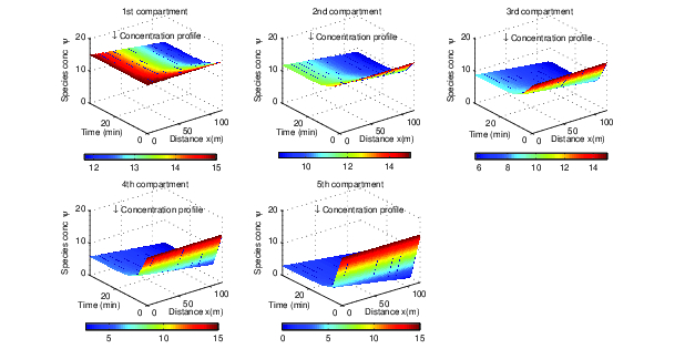
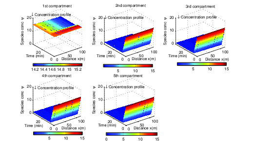
Figure 2. Species concentration profile for linear boundary sinks \(\beta = 1\) of interconnected (m=5)multiple-compartment system at time t = 36 mins.Figure 3. Species concentration profile for nonlinear boundary sinks \(\beta = 2\) of interconnected (m=5)multiple-compartment system at time t = 36 mins.Figure 4. Species concentration profile for nonlinear boundary sinks \(\beta = 7\) of interconnected (m=5)multiple-compartment system at time t = 36 mins.
From Figure 2 for linear boundary sink \(\beta = 1\) at time t=36 minutes, end of one boundary and the beginning of another boundary of each compartment of the system maintains the same concentration values of 11.77 mg/L, 8.70 mg/L, 5.75 mg/L, 2.86 mg/L and 0.00 mgL respectively. However, there is a significant drop in the concentration profile for nonlinear boundary sink \(\beta = 2\) between the end of one compartment and the beginning of another compartment as they do not maintain the same concentration profile at the boundaries of the compartments for the chemical species being transported through the interconnected multiple-compartment system as shown in Figure 3. The values of the concentration at t=36 minutes are 14.17 mg/L, 3.08 mg/L, 1.10 mg/L, 0.41 mg/L and 0.00 mgL which are obtained at the boundary end of each compartment of the reactor system.
For strongly nonlinear boundary sink \(\beta = 7\) depicted in Figure 4, more drop of the concentration profile is observed. The values of the species concentration at the boundary end of each compartment are 14.15 mg/L, 0.73 mg/L, 0.24 mg/L, 0.10 mg/L and 0.00 mgL respectively at t = 36 minutes.
While results from Figure 1 indicate a small drop in concentration profile to 10.22 mg/L at mid-point of the second compartment for linear boundary sink \(\beta = 1\) , results from Figures 2 and 3 at the mid-point of the second compartment for nonlinear boundary sinks \(\beta = 2\) and \(\beta = 7\) show significant drop in concentration values to 3.42 mg/L and 1.09 mg/L respectively. Generally , this means that whenever a chemical species with linear sinks (first order chemical reaction kinetic decay) is transported through adjacent compartments of interconnected multiple-compartment system, there is significant drop in concentration profile at the adjacent compartments as nonlinear boundary sinks increase.
5. Conclusion
The emphasis in this research work is on investigating the influence of nonlinearity at the boundaries on the concentration profile of a chemical species being transported – in adjacent compartments – through multiple-compartment isothermal system. The system is such that each compartment is connected with form of sieve partitions allowing nonlinear sinks at such boundaries. Comparison was made between linear boundary sink \(\beta = 1\) as shown in Figure 2 and nonlinear boundary sinks \(\beta = 2\) and \( 7 \) as shown in Figures 3 and 4.
The results show that for strongly nonlinear boundary sinks, the concentration profile at the adjacent compartments significantly dropped to very low values in the interconnected multiple-compartment system. Hence interconnected multiple-compartment systems with strongly nonlinear boundary sinks may not be suitable for systems where high concentration profile in adjacent compartment is needed. Therefore, we recommend such models for system designs in which low concentration profile is the target.
Acknowledgments
The authors wish to express their profound gratitude to the reviewers for their useful comments.
Author Contributions
All authors contributed equally to the writing of this paper. All authors read and approved the final manuscript.
Conflict of Interests
The authors declare no conflict of interest.
References
Chick, H. (1908). An investigation of the laws of disinfection. Epidemiology & Infection, 8(1), 92-158. [Google Scholor]
Igbokwe, P. K., Nwabanne, J. T., & Gadzama, S. W. (2015). Characterization of a 5 litre continuous stirred tank reactor. World Journal of Engineering and Technology, 3(02), 25.
[Google Scholor]
Watson, H. E. (1908). A note on the variation of the rate of disinfection with change in the concentration of the disinfectant. Epidemiology & Infection, 8(4), 536-542.
[Google Scholor]
Critelli, R. A., Bertotti, M., & Torresi, R. M. (2018). Probe effects on concentration profiles in the diffusion layer: Computational modeling and near-surface pH measurements using microelectrodes. Electrochimica Acta, 292, 511-521.
[Google Scholor]
Gu, J. J., & Wang, J. M. (2019). Sliding mode control for N-coupled reaction-diffusion PDEs with boundary input disturbances. International Journal of Robust and Nonlinear Control, 29(5), 1437-1461.
[Google Scholor]
Karafyllis, I., Krstic, M., & Chrysafi, K. (2019). Adaptive boundary control of constant-parameter reaction-diffusion PDEs using regulation-triggered finite-time identification. Automatica, 103, 166-179.
[Google Scholor]
Orava, V., Soucek, O., & Cendula, P. (2015). Multi-phase modeling of non-isothermal reactive flow in fluidized bed reactors. Journal of Computational and Applied Mathematics, 289, 282-295.
[Google Scholor]
Schulz, R., Yamamoto, K., Klossek, A., Rancan, F., Vogt, A., Schütte, C., … & Netz, R. R. (2019). Modeling of drug diffusion based on concentration profiles in healthy and damaged human skin. Biophysical Journal, 117(5), 998-1008.
[Google Scholor]
Sharma, A. K., Birgersson, E., & Vynnycky, M. (2015). Towards computationally-efficient modeling of transport phenomena in three-dimensional monolithic channels. Applied Mathematics and Computation, 254, 392-407.
[Google Scholor]
Wang, S., & Linsenmeier, R. A. (2007). Hyperoxia improves oxygen consumption in the detached feline retina. Investigative Ophthalmology & Visual Science, 48(3), 1335-1341. [Google Scholor]
Cougnon, P., Dochain, D., Guay, M., & Perrier, M. (2006). Real-time optimization of a tubular reactor with distributed feed. Journal of Amerasian Institute of Chemical Engineering , 52(6), 2120-2128.
[Google Scholor]
Lu, Y., Dixon, A. G., Moser, W. R., & Ma, Y. H. (1997). Analysis and optimization of cross-flow reactors with staged feed policies-isothermal operation with parallel-series, irreversible reaction systems. Chemical Engineering Science, 52(8), 1349-1363.
[Google Scholor]
Hamel, C., Thomas, S., Schädlich, K., & Seidel-Morgenstern, A. (2003). Theoretical analysis of reactant dosing concepts to perform parallel-series reactions. Chemical Engineering Science, 58(19), 4483-4492.[Google Scholor]
Nocon, W. (2006). Mathematical modelling of distributed feed in continuous sedimentation. Simulation Modelling Practice and Theory, 14(5), 493-505.[Google Scholor]
Rostami, F., Shahrokhi, M., Said, M. A. M., & Abdullah, R. (2011). Numerical modeling on inlet aperture effects on flow pattern in primary settling tanks. Applied Mathematical Modelling, 35(6), 3012-3020.
[Google Scholor]
Adedire, O., & Ndam, J. N. (2019). Mathematical modeling of chlorine decay through water and intermediate pseudomonas aeruginosa in multiple-compartment isothermal reactor. Journal of Advanced Mathematical Models and Applications, 4(2), 167-178.
[Google Scholor]
Adedire, O., and Ndam, J. N. (2020). Mathematical modelling of concentration profiles for species transport through the single and the interconnected multiple-compartment systems. Journal of the Nigerian Society of Physical Sciences, 2, 61-68.
[Google Scholor]
Strikwerda, J. (1977). Initial boundary value problems for incomplete parabolic systems. Journal of Communications on Pure and Applied Mathematics, 30, 797-822.
[Google Scholor]
Thompson, P.A. (1972). Compressible-fluid dynamics. New York: McGraw-Hill, Inc.
[Google Scholor]
Tyrrell, H. J. V. (1964). The origin and present status of Fick’s diffusion law. Journal of Chemical Education, 41(7), 397.
[Google Scholor]
Crank, J. (1979). The mathematics of diffusion. Oxford university press.
[Google Scholor]
Kreiss, H., and Lorenz, J. (1989). Initial-boundary value problems and the Navier-Stokes Equation. San Diego: Academic Press, Inc.
[Google Scholor]