This paper presents the development of a new numerical scheme for the solution of exponential growth and decay models emanated from biological sciences. The scheme has been derived via the combination of two interpolants namely, polynomial and exponential functions. The analysis of the local truncation error of the derived scheme is investigated by means of the Taylor’s series expansion. In order to test the performance of the scheme in terms of accuracy in the context of the exact solution, four biological models were solved numerically. The absolute error has been computed successfully at each mesh point of the integration interval under consideration. The numerical results generated via the scheme agree with the exact solution and with the fifth order convergence based upon the analysis carried out. Hence, the scheme is found to be of order five, accurate and is a good approach to be included in the class of linear explicit numerical methods for the solution of initial value problems in ordinary differential equations.
Keywords: Accuracy, biological model, ordinary differential equation, initial value problem, local truncation error.
1. Introduction
Differential equations are useful to modern science and engineering. Differential equation models are used extensively in biology to study biochemical reactions, population dynamics, organism growth, and the spread of diseases. The most common use of differential equations in science is to model dynamical systems. Such physical models represent future estimation for any real world situation based on the data available in the past and present as detailed in [1,2,3,4,5,6,7,8,9].
However, these models are said to have no closed form solution in most of the real cases. In such situations, one has to compromise at numerical approximate solutions of the models achievable by various numerical techniques of different characteristics [10]. Development of new numerical integration methods with varying characteristics for the solution of initial value problems in ordinary differential equations has attracted the attention of many researchers in past and recent years as detailed in [11,12,13,14,15,16,17].
The main aim of the paper is to develop a new numerical method of order five via the combination of two interpolants for its possible acceptance within the class of linear explicit numerical techniques. Also the local truncation errors and order of accuracy of the scheme were thoroughly investigated. The rest of the paper is structured as follows; Section 2 presents the development of the scheme. In Section 3, the local truncation error of the scheme has been investigated. Also the order of accuracy of the scheme is obtained. Section 4 presents numerical experiments, discussion of results and concluding remarks.
where \(\beta_{0}, \beta_{2}, \beta_{3}, …, \beta_{6} \) are undetermined constants and \(c \) is a constant.
The integration interval of \([a, b] \) is defined as
respectively.
Differentiating (6) five times and using the fact that
\[F'(x_{n}) = f_{n}, F”(x_{n}) = f^{(1)}_{n}, F”'(x_{n}) = f^{(2)}_{n}, F^{(iv)}(x_{n}) = f^{(3)}_{n}, F^{(v)}(x_{n}) = f^{(4)}_{n} \] yields
Equation (46) shows that the order of the scheme is five.
Remark 1.
The local truncation error of the scheme is summarized in the following result.
Theorem 1.
By means of the Taylor’s series expansion and the localizing assumption, the scheme given by (40) has fifth order accuracy.
4. Numerical experiments, discussion of results and concluding remarks
The developed scheme was derived via the combination of two interpolants namely polynomial function and trigonometric function via MAPLE 18. The scheme (40) was implemented on biological models with the aid of MATLAB R2014a (8.3.0.532), 32-bit (Win 32) programming language.
4.1. Numerical experiments
Biological models that find applications in science in terms of modelling growth and decay shall be considered. The scheme (40) is implemented on these models and the results obtained were compared with the exact solutions.
Experiment 1.
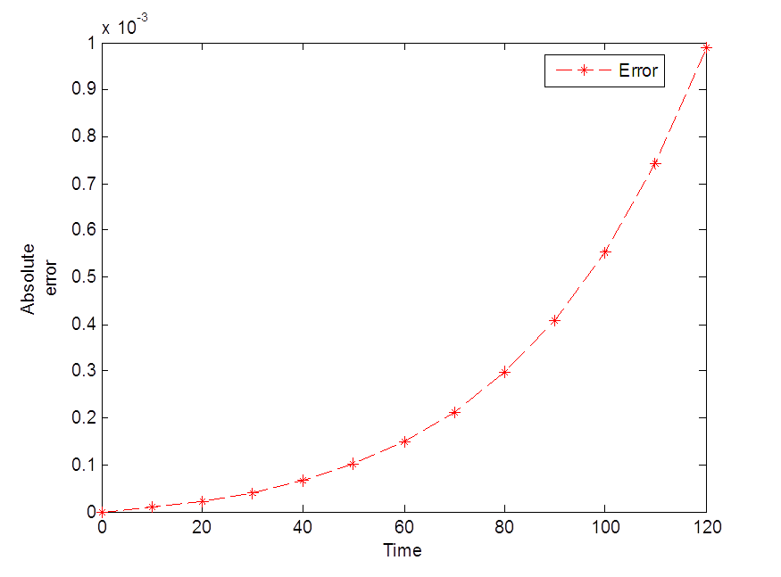
Assume that a colony of 100 bacteria is multiplying at the rate of \(k=0.02 \) per hour per individual. How many bacteria are there after 120 minutes? It is assumed that the colony grows continuously and without restriction.
Here, it is evident that the rate of population growth is proportional to the size of population. It is possible to model this exponential growth with an initial value problem of first order ordinary differential equation of the form
\begin{equation}
\label{47}
\frac{dp}{dt} = kp, p(0) = 100, k = 0.02, 0\leq t \leq 120,
\end{equation}
(47)
where \(p=p(t) \) is the population of the bacteria, \(p(0)=p_{0} \) is the initial population of the bacteria, \(t \) is the time and \(k \) is the growth rate.
The exact solution of (47) is obtained as
The comparative results analysis of the scheme (40) \(”p_{n}”\) and the exact solution \(”p(t_{n})”\) with \(h = 10 \) are shown in Table 1.
Table 1. The results generated via the scheme (40) and the exact solution.
\(n \)
\(t_{n} \)
\(p_{n} \)
\(p(t_{n}) \)
\(e_{n} = \vert p(t_{n})-p_{n} \vert \)
0.00
0.00
100.0000000000
100.0000000000
0.0000000000
1.00
10.00
122.1402666667
122.1402758160
0.0000091494
2.00
20.00
149.1824474140
149.1824697641
0.0000223501
3.00
30.00
182.2118390914
182.2118800391
0.0000409477
4.00
40.00
222.5540261644
222.5540928492
0.0000666848
5.00
50.00
271.8280810347
271.8281828459
0.0001018113
6.00
60.00
332.0115430506
332.0116922737
0.0001492230
7.00
70.00
405.5197840461
405.5199966845
0.0002126383
8.00
80.00
495.3029456200
495.3032424395
0.0002968195
9.00
90.00
604.9643385882
604.9647464413
0.0004078531
10.00
100.00
738.9050563898
738.9056098931
0.0005535033
11.00
110.00
902.5006062880
902.5013499434
0.0007436554
12.00
120.00
1102.3166471884
1102.3176380642
0.0009908757
Figure 1. Errors generated via the scheme (40).
Experiment 2.
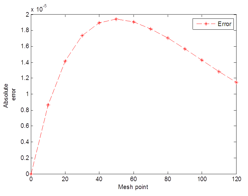
Consider the exponential decay model of the form
\begin{equation}
\label{49}
\frac{dp}{dt} = -rp, p(0) = 100, r =0.02, 0\leq t \leq 120,
\end{equation}
(49)
where \(p=p(t) \) is the population of the bacteria, \(p(0)=p_{0} \) is the initial population of the bacteria, \(t \) is the time and \(r \) is the decay rate.
The exact solution of (49) is obtained as
The comparative results analysis of the scheme (40) \(”p_{n}”\) and the exact solution \(”p(t_{n})”\) with \(h = 10 \) are shown in Table 2.
Table 2. The results generated via the scheme (40) and the exact solution.
\(n \)
\(t_{n} \)
\(p_{n} \)
\(p(t_{n}) \)
\(e_{n} = \vert p(t_{n})-p_{n} \vert \)
0.00
0.00
100.0000000000
200.0000000000
0.0000000000
1.00
10.00
81.8730666667
81.8730753078
0.0000086411
2.00
20.00
67.0319904540
67.0320046036
0.0000141495
3.00
30.00
54.8811462324
54.8811636094
0.0000173770
4.00
40.00
44.9328774423
44.9328964117
0.0000189694
5.00
50.00
36.7879247036
36.7879441171
0.0000194135
6.00
60.00
30.1194021179
30.1194211912
0.0000190734
7.00
70.00
24.6596781756
24.6596963942
0.0000182186
8.00
80.00
20.1896347525
20.1896517995
0.0000170470
9.00
90.00
16.5298731206
16.5298888222
0.0000157015
10.00
100.00
13.5335140400
13.5335283237
0.0000142837
11.00
110.00
11.0803029723
11.0803158362
0.0000128639
12.00
120.00
9.0717838394
9.0717953289
0.0000114896
Figure 2. Errors generated via the scheme (40).
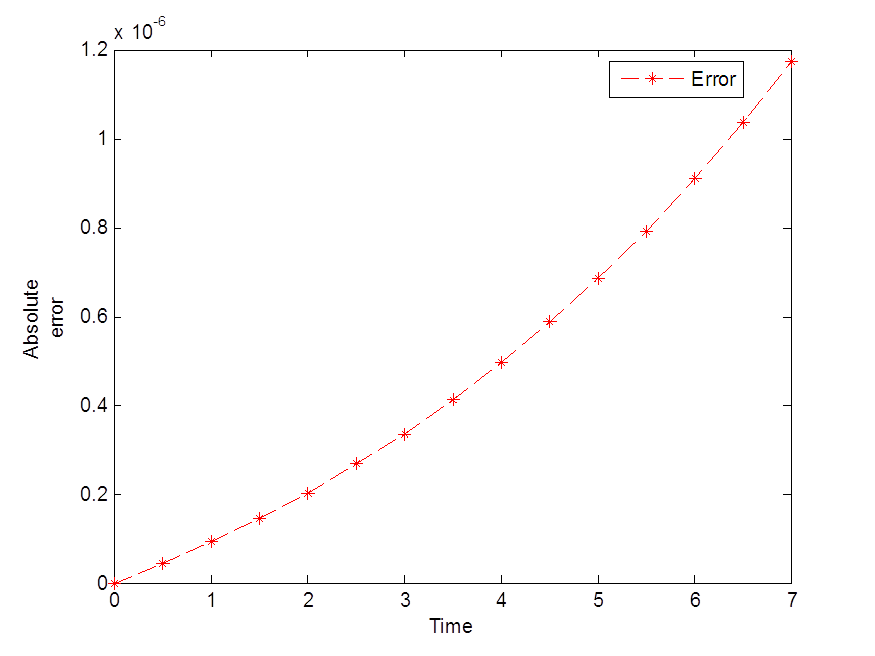
Experiment 3. [19]
Suppose there are 1000 birds on an Island, breeding with a constant continuous growth rate of \(10% \) per year. But now birds migrate to the Island at a constant rate of 100 new arrivals per year. How many birds are on the Island after seven years?
Let \(p=p(t) \) be the number of birds on Island, \(t \) is the time, \(k \) is a constant continuous growth rate, \(m \) be the rate of migration of the population. The model equation for population growth with migration is given by
\begin{equation}
\label{51}
\frac{dp}{dt} = kp + m, p(0) = 1000, k = 0.1, m = 100, 0\leq t \leq 7.
\end{equation}
The comparative results analysis of the scheme (40) \(”p_{n}”\) and the exact solution \(”p(t_{n})”\) with \(h = 0.5 \) are shown in Table 3.
Table 3. The results generated via the scheme (40) and the exact solution.
\(n \)
\(t_{n} \)
\(p_{n} \)
\(p(t_{n}) \)
\(e_{n} = \vert p(t_{n})-p_{n} \vert \)
0.00
0.00
1000.0000000000
1000.0000000000
0.0000000000
1.00
0.50
1102.5421927083
1102.5421927520
0.0000000437
2.00
1.00
1210.3418360594
1210.3418361513
0.0000000919
3.00
1.50
1323.6684853116
1323.6684854566
0.0000001449
4.00
2.00
1442.8055161172
1442.8055163203
0.0000002032
5.00
2.50
1568.0508331085
1568.0508333755
0.0000002670
6.00
3.00
1699.7176148152
1699.7176151520
0.0000003368
7.00
3.50
1838.1350967735
1838.1350971865
0.0000004131
8.00
4.00
1983.6493947863
1983.6493952825
0.0000004963
9.00
4.50
2136.6243703934
2136.6243709803
0.0000005869
10.00
5.00
2297.4425407147
2297.4425414003
0.0000006856
11.00
5.50
2466.5060349420
2466.5060357348
0.0000007928
12.00
6.00
2644.2375998718
2644.2376007810
0.0000009092
13.00
6.50
2831.0816569923
2831.0816580278
0.0000010355
14.00
7.00
3027.5054137686
3027.5054149410
0.0000011723
Figure 3. Errors generated via the scheme (40).
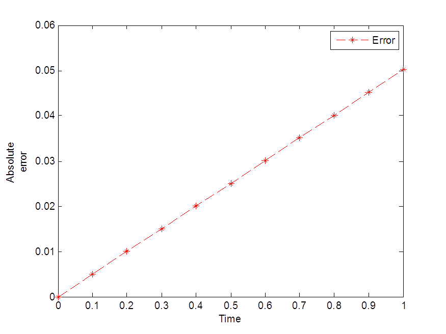
Experiment 4. [19]
A cell culture in a biology laboratory currently holds 1000000 cells. The cells have a constant continuous birth rate of \(1.5% \) and death rate of \(0.5% \) per hour. Cells are extracted from the culture for an experiment at the rate of 5000 per hour. How many cells will be in the culture 1 hour from now?
Let \(p=p(t) \) be the population, \(t \) be the number of hours from now, \(k \) be the difference between the birth rate and death rate, \(b \) be the birth rate, \(d \) be the death rate and \(n \) be the extracted cells. The model equation for the growth and decay with input and output is given by
$$\frac{dp}{dt} = (b-d)p + n, p(0) = 1000000, 0\leq t \leq 1,$$
(53)
where \(b=0.015, d = -0.005, k = 0.01, n = -5000 \). The exact solution of (53) is obtained as
The comparative results analysis of the scheme (40) \(”p_{n}”\) and the exact solution \(”p(t_{n})”\) with \(h=0.1 \) are shown in Table 4.
Table 4. The results generated via the scheme (40) and the exact solution.
\(n \)
\(t_{n} \)
\(p_{n} \)
\(p(t_{n}) \)
\(e_{n} = \vert p(t_{n})-p_{n} \vert \)
0.00
0.00
1000000.0000000000
1000000.0000000000
0.0000000000
1.00
0.10
1000500.2550850213
1000500.2500833542
0.0050016671
2.00
0.20
1001001.0106753386
1001001.0006670002
0.0100083384
3.00
0.30
1001502.2672717074
1001502.2522516886
0.0150200188
4.00
0.40
1002004.0253753845
1002004.0053386709
0.0200367136
5.00
0.50
1002506.2854881278
1002506.2604297005
0.0250584274
6.00
0.60
1003009.0481121978
1003009.0180270325
0.0300851653
7.00
0.70
1003512.3137503569
1003512.2786334243
0.0351169326
8.00
0.80
1004016.0829058710
1004016.0427521367
0.0401537343
9.00
0.90
1004520.3560825090
1004520.3108869339
0.0451955751
10.00
1.00
1005025.1337845444
1005025.0835420840
0.0502424604
Figure 4. Errors generated via the scheme (40).
4.2. Summary of the results
The summary of the results generated via the scheme and the exact solution at the final mesh point time in the nearest whole number is presented as follows (Table 5):
4.2. Summary of the results
The summary of the results generated via the scheme and the exact solution at the final mesh point time in the nearest whole number is presented as follows (Table 5):
Table 5. The summary of the accuracy of results generated via the scheme (40) against exact solution.
Experiments
\(t_{nfl} \)
\(p_{nfl} \)
\(p(t_{nfl}) \)
\(e_{nfl} = \vert p(t_{n}fl)-p_{nfl} \vert \)
Experiment 1
120 mins.
1102
1102
0.000
Experiment 2
120 mins.
9
9
0.0000
Experiment 3
7 hours
3027
3027
0.0000
Experiment 4
1 hour
1005025
1005025
0.0000
4.3. Discussion of results and concluding remarks
In this paper, a new fifth order scheme for the solution of initial value problems in ordinary differential equations emanated from biological sciences is developed via the combination of two interpolants. Four numerical experiments have been performed to test the performance of the scheme in terms of the accuracy in the context of the exact solution as shown in Tables 1-4 and also absolute errors computed at each mesh point of the integration interval under consideration as demonstrated in Figures 1-4. The numerical results in Tables 1-4 show that the fifth order scheme is accurate and converges faster to the exact solution. The effect of the constant \(k \) determines the solution of the models under consideration. It is observed from Tables 1, 3 and 4 that the results of the scheme and the exact solution increase exponentially over time. It is also observed from Table 2 that the results of both the scheme and the exact solution decrease over time. When compared with the exact solutions, the fifth order scheme yielded smaller amount of errors as seen from the above Figures 1-4. The summary of the results generated via the fifth order scheme in the context of the exact solution is presented in Table 5. Hence, the fifth order scheme is a good approach to be included in the class of linear explicit numerical methods as its analysis carried out agrees with the exact solution of exponential growth and decay models emanated biological sciences. Finally, all the calculations were carried out via MATLAB R2014a, Version: 8.3.0.552, 32 bit (Win 32) in double precision.
Conflicts of interest
”The author declares no conflict of interest.”
References
Ansari, M. Y., Shaikh, A. A., & Qureshi, S. (2018). Error bounds for a numerical scheme with reduced slope evaluations. Journal of Applied Environmental and Biological Sciences, 8(7), 67-76. [Google Scholor]
Bird, J. (2017). Higher Engineering Mathematics. Taylor and Francis Group, London. [Google Scholor]
Butcher, J. C. (2016). Numerical Methods for Ordinary Differential Equations. John Wiley and Sons, Ltd., United Kingdom. [Google Scholor]
Jain, M. K. (2003). Numerical Methods for Scientific and Engineering Computation. New Age International (P) Ltd., New Delhi, India. [Google Scholor]
Lambert, J. D. (1991). Numerical Methods for Ordinary Differential Systems: the Initial Value Problem. John Wiley and Sons, Inc., New York. [Google Scholor]
Lambert, J. D. (2011). Computational Methods in Ordinary Differential Equations. John Wiley and Sons Inc. [Google Scholor]
Rabiei, F., & Ismail, F. (2011). Third-order Improved Runge-Kutta method for solving ordinary differential equation. International Journal of Applied Physics and Mathematics, 1(3), 191-194. [Google Scholor]
Applications of Differential Equations. http://faculty.bard.edu/belk/math213s14, accessed on April 27, 2020. [Google Scholor]
Zill, D. G. (2012). A First Course in Differential Equations with Modeling Applications. Cengage Learning. [Google Scholor]
Qureshi, S., & Emmanuel, F. S. (2018). Convergence of a numerical technique via interpolating function to approximate physical dynamical systems. Journal of Advanced Physics, 7(3), 446-450. [Google Scholor]
Fadugba, S. E., & Idowu, J. O. (2019). Analysis of the properties of a third order convergence numerical method derived via transcendental function of exponential form. International Journal of Applied Mathematics and Theoretical Physics, 5(4), 97-103. [Google Scholor]
Ogunrinde, R. B., & Fadugba, S. E. (2012). Development of a new scheme for the solution of initial value problems in ordinary differential equations. International Organization of Scientific Research Journal of Mathematics (IOSRJM), 2, 24-29. [Google Scholor]
Fadugba, S. E., & Okunlola, J. T. (2017). Performance measure of a new one-step numerical technique via interpolating function for the solution of initial value problem of first order differential equation. World Scientific News, 90, 77-87. [Google Scholor]
Fadugba, S. E., & Olaosebikan, T. E. (2018). Comparative study of a class of one-step methods for the numerical solution of some initial value problems in ordinary differential equations. Research Journal of Mathematics and Computer Science, 2(9), 1-11. [Google Scholor]
Qureshi, S., Shaikh, A. A., & Chandio, M. S. (2019). A new iterative integrator for Cauchy problems. Sindh University Research Journal-SURJ (Science Series), 45(3). [Google Scholor]
Rabiei, F., & Ismail, F. (2012). Fifth-order Improved Runge-Kutta method for solving ordinary differential equation. Australian Journal of Basic and Applied Sciences, 6(3), 97-105. <a href="https://scholar.google.com/scholar?hl=en&as_sdt=0%2C5&q=Fifth-order+Improved+Runge-Kutta+method+for+solving+ordinary+differential+equation.+[Google Scholor]
Fadugba, S. E. & Qureshi, S. (2019). Convergent numerical method using transcendental function of exponential type to solve continuous dynamical systems. Punjab University Journal of Mathematics, 51(10), 45-56. [Google Scholor]
Brown, P., Evans, M., & Hunt, D. (2013). Growth and decay-A guide for teachers (Years 11-12). Educational Services, Australia. [Google Scholor]