Mathematical analysis of a delayed HIV/AIDS model with treatment and vertical transmission

1. Introduction

Apart from covid-19, HIV/AIDS has attracted more attention worldwide as it has been a big disease that killed a large number of human being around the globe. HIV/AIDS is still lingering in society, it has not been eradicated as well. The only solution is all about the preventive measures to make it delay. Many of existing infectious diseases are transmitted through both vertical and horizontal modes for instance AIDS, hepatitis B, rubella and more just to mention few [1,2]. Infected hosts persist in a dormant period before they become infectious [3,4].

In the history of human beings, communicable diseases killed many and left a lot of vulnerable with various consequences. This cause a global concern in order to mitigate some of the effects of those diseases. AIDS was first reported in America in 1981 [5]. It is a fatal illness that disintegrates the human immune system, leaving the victim exposed, threatening infectious diseases, neurological disorders or unexpected malignancies. It causes the deaths of millions of people and a huge amount of money spent on health care and disease management. It was estimated that there was 38.6 million people and 2.8 million AIDS death in 2005 [6], while 39.5 million people in the world were living with HIV, 4.3 million new infections and 2.9 million of people died of AIDS-related diseases in 2006 [7]. Approximately 36.7 million people worldwide were living with HIV/AIDS at the end of 2015 [8] and about 36.9 million people in 2017 where 66% of all new HIV infections found in sub-Sahara Africa [9]. Then 37 million people in 2018 [10]. This shows that HIV/AIDS is still there and active. The world is preoccupied with the global pandemic covid-19, but HIV/AIDS continues to kill a significant proportion of individuals and has resulted in an increase in the number of orphans and helpless group of people. HIV/AIDS is a complicated disease caused by human immunodeficiency virus infection [11]. This HIV attacks the CD4 receptor to connect and enter the lymphocyte [12]. A healthy person, the level of \(CD4^{+}\)T cells is between 800 and \(1200 / mm^{3}\), once this number reaches 200 or less in an HIV infected patient, the person is identified as having AIDS [13]. The infected person can live longer through infective stages before developing AIDS [14]. The modes of transmission of HIV virus are mainly unprotected sex, through the exchanging of infected needles, infected blood transfusion from mother to child i.e., vertical transmission [15]. By studying the stability analysis, one could know when and where the disease spreads using the basic reproduction number [16]. It is regarded to be the limit quantity representing whether the disease spreads or ends up dead in the susceptible population.

Some different observations have been made to analyze the HIV/AIDS dynamics without delay [17,18]. However, few studies have been conducted on effect of time delays [19,20]. HIV is normally transmitted in two basic modes namely horizontal transmission and vertical transmission. [8] presented the spread of disease only by horizontal transmission while [21,22,23] studied a delayed HIV/AIDS model considering vertical transmission. Delay approaches provide good functionality with reality as they capture the dynamics from the onset of diagnosis to infection [21,24,25]. HIV/AIDS can be delayed by taking antiretroviral drugs, which are prescribed to manage HIV, and slow the replication of the virus and significantly delay the progression to AIDS.

HIV is transmitted by direct contact between the mucous membranes or bloodstream with HIV-containing body fluids, such as pre-seminal fluid, blood, vaginal fluid, semen, and breast milk [26]. It can be successfully transmitted to the closed society [27]. Preventive strategies such as abstinence, fidelity and condom use have resulted in a modest decline in HIV prevalence, especially in close communities, such as commercial sex workers and their clients [28]. The HIV virus attacks immune cells, which are called T-helper cells or CD4 cells. These are critical when it comes to maintaining a healthy immune system as they fight against diseases and infections. HIV cannot grow or reproduce itself. Instead, it makes new copies of itself inside T-helper cells that damage the immune system and gradually weaken the natural body defense. This process of T-helper cell multiplication is called the HIV life cycle. How quickly the virus develops depends on how early you are diagnosed, your overall health, and how well you are taking your treatment. It is useful to know that antiretroviral drugs keep the immune system healthy if they are taken correctly.

Most people who are infected with HIV have been able to carry the virus for years before any severe symptoms develop. But over time, the level of HIV in the blood increases, while the number of \(CD4+\) \(T\) cells decreases. Antiretroviral medicines can help in reducing the amount of virus in the body to preserve \(CD4+\) \(T\) cells and dramatically slow the destruction of the immune system.

There are many factors that could delay the time between HIV and AIDS, which include taking antiretroviral treatment consistently, staying in regular HIV care, adhering closely to your doctor's advice, eating healthy foods, taking care of yourself and your genetic background. As HIV/AIDS kills a huge number of people every year, it is crucial to conduct this study in order to access mathematical analysis of a delayed HIV/AIDS model with treatment and vertical transmission when a pre-AIDS group is considered.

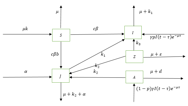
According to [21] model AIDS patients are isolated which is impossible in real world situation as many of them are still being in services and they are experts in various domains. In this study, a high number of symptomatic infections \((J)\) where patients know very well their health status is considered, because this can help them to take some measures regarding giving birth and the number of newborns infected children can be limited as well. In case HIV/AIDS patients are from asymptomatic group \((I)\) where they do not know their health status and still joining AIDS group without any information, the newly born infected children should increase dramatically. This number is assumed to be small in the present model. This present paper, adds a pre-AIDS group to the model introduced by [21]. We divided the total populations \(N(t)\) into five classes such as : The susceptible group \((S)\), The asymptomatic infectives or unaware HIV infected group \((I)\), The symptomatic infective or aware \(HIV\) infected group \((J)\), pre AIDS class \((Z)\) and AIDS class or Full-blown AIDS group \((A)\).

The structure of the paper is as follows: the Section 2 is the model formulation, Section 3 represents model analysis which consists of positivity and boundedness, Basic reproduction number, stability analysis, local stability of disease free equilibrium, global stability of disease free equilibrium, global stability of endemic equilibrium, Section 4 represents numerical results and discussion, and Section 5 represents conclusion and recommendation.

2. Model formulation

Cai et al., [6] represented local and global stability of the equilibria of a \(SIJA\) model with treatment. Authors assumed that some individuals with the symptomatic phases \((J)\) can be transformed into asymptomatic individuals \((I)\) after treatment. Naresh et al., [24] studied \(SIA\) model with vertical transmission, assuming that a fraction of newborns, who sustain treatment joint the infective class while others who do not sustain treatment, join the AIDS class after getting sexual maturity. Osman et al., [21] proposed an HIV/AIDS model which incorporates time delay and vertical transmission, considered a newly born infected child attains sexual maturity and becomes infectious. It was assumed that asymptomatic infectives \((J)\) have the symptoms of AIDS, AIDS patients \((A)\) are isolated hence their probability of producing children is small, and it is neglected.

Referring to the \(SIJA\) Model with treatment introduced by Cai et al., [6] written as:

And \(SIA\) Model with vertical transmission proposed by Naresh et al., [24] which is presented as: Then, from (1) and (2), Osman et al., [21] ameliorated the model and came up with stability analysis of a delayed HIV/AIDS epidemic model with treatment and vertical transmission as follows: In the model (3), authors considered AIDS patients (A) to be isolated hence their probability of producing children is very small and it is neglected but still to isolate people with HIV cannot be easy. It is impossible in society as many of them serve society in different domains like Education, Leadership, Army, Physicians, and so on. To solve this problem, we propose the model which consider high number of people who know their health status (J) and this can decrease the probability of infected newborn and reduce the spread of infection. We also added the Pre-AIDS group from [8] to the model (3) in order to evaluate the behaviour and stability of the model. According to [8] the following model was explored: The following nonlinear dynamic equation system was derived from the model (3) and (4) respectively: subjected to the initial conditions \( S= S_0\geq0\), \(I = I_0 \geq0\), \(J=J_0 \geq0\), \(Z= Z_0\geq0\), \(A = A_0 \geq0\).

2.1. Model presentation

In this section, we develop a compartmental model of delayed HIV/AIDS treatment and vertical transmission epidemic, including pre-AIDS class. Based on the epidemiological status, the population is divided into five groups, as pointed out earlier. We can represent the diagram of a delayed HIV/AIDS model as (Figure 3):

The variables and parameters in the model (5) are described in Table 1.

Table 1. Description of variables and parameters of the model.

Parameters	Description
\(S\)	The susceptibles
\(I\)	The asymptomatic infectives (un-aware)
\(J\)	The symptomatic infectives (aware)
\(Z\)	The pre-AIDS group
\(A\)	The Full-blown AIDS group (AIDS class)
\(\gamma\)	The birth rate of infected newborns
\(k\)	The  recruitment rate of the population
\(\mu\)	The death rate
\(c\)	The average number of contacts of an individual per unit of time
\(\beta\)	The probability of disease transmission per contact by an infective in the first stage
\(b\)	The probability of disease transmission per contact by an infective in second stage
	by an infective in the first stage and in the second stage
\(k_{1}\)	The rate from the asymptomatic phase \((I)\) to the symptomatic phase \((J)\)
\(k_{2}\)	The rate from the symptomatic phase \(J\) to the AIDS cases \(A\)
\(k_{3}\)	The transfer rate of asymptomatic phase \((I)\) ( un-ware)  to AIDS group \(A\)
\(\alpha\)	The transformation rate from the symptomatic phase \((J)\) to asymptomatic phase \((I)\)
\(d\)	The disease related death rate of the AIDS cases
\(p\)	The fraction of infected newborns joining the asymptomatic infective class after getting sexual maturity
\(\epsilon\)	The AIDS related death rate
\(t\)	The time
\(\tau\)	Length in delay

3. Model analysis

The analysis focuses on how to obtain the basic reproduction number, the point of the free disease (non-endemic) and its stability, and the point of the endemic disease and its stability. In this section, we find the fundamental properties of the system (5), which is important in the proof of the following sections.

3.1. Positivity and boundedness

The associated parameters in (5) with respect to the original conditions are non-negative for all \(t > 0 \) and this is shown in the following procedures:

Lemma 1. If \({S(0), I(0), J(0), Z(0), A(0)}\) and all parameters of the system are positive, then solutions \(S(t)\), \(I(t)\), \(J(t)\), \(Z(t)\), \(A(t)\) are all positive \(\forall\); \(t > 0\).

Proof. Let \( t_{1} = \sup \left\lbrace t > 0 \left| S(t) \geq 0, I(t) \geq 0, J(t) \geq 0, Z(t)\geq0, A(t) \geq 0\right. \right\rbrace\). The first equation in (5) yields \begin{equation*} \frac{dS}{dt}= \mu k-c\beta[I(t)+bJ(t)]S(t)-\mu S(t). \end{equation*} Since \(\mu k\geq0\), then \( \frac{dS}{dt}\geq-(\mu+\omega)S,\) where \(\omega=[c\beta(I(t)+bJ(t))] \) yields \begin{align*} &\int_{o}^{t_{1}}\frac{dS}{S}= -\int_{0}^{t_{1}}(\mu+\omega)dt,\\ &\ln|S(t)|_{0}^{t_{1}} \geq -(\mu+\omega)t_{1},\\ &|S(t)|_{0}^{t_{1}} \geq e^{-(\mu+\omega)t_{1}},\\ & S(t) \geq S(0)+e^{-(\mu+\omega)t_{1}}>0. \end{align*} Next, we prove that \(I(t) > 0\). The second equation in (5) gives \begin{equation*} \frac{dI}{dt}=\omega S(t)-(\mu+k_1 )I(t)+\alpha J(t)+\gamma pI(t-\tau)e^{-\mu\tau}. \end{equation*} Since \((\omega S+\alpha J)\geq0\), then \begin{equation*} \frac{dI}{dt}\geq-\left[(\mu+k_1 )+\gamma p(\tau -t) e^{-\mu \tau}\right]I. \end{equation*} Integrating both sides yields, \begin{align*} \int_{o}^{t_{1}}\frac{dI}{I}=&- \int_{0}^{t_{1}}\left[(\mu+k_1 )+\gamma p(\tau -t) e^{-\mu \tau}\right]dt\\ = &-\int_{o}^{t_{1}}\left[(\mu+k_1 )+ \gamma p \tau e^{-\mu \tau}\right]dt + \int_{o}^{t_{1}} \gamma p t e^{-\mu \tau}dt\\ = & \left|-\left[(\mu+k_{1})+\gamma p \tau e^{-\mu \tau}\right]t\right|_{0}^{t_{1}}+\left|\gamma p e^{-\mu \tau}\frac{t^{2}}{2}\right|_{0}^{t_{1}}\\ = &-\left[\left((\mu+k_{1})+\gamma p \tau e^{-\mu \tau}\right) -\gamma p e^{-\mu \tau}\frac{t_{1}}{2}\right]t_{1},\\ \ln|I(t)|_0^{t_1 } \geq & -\left[\left((\mu+k_{1})+\gamma p \tau e^{-\mu \tau}\right) -\gamma p e^{-\mu \tau}\frac{t_{1}}{2}\right]t_{1},\\ |I(t)|_0^{t_1 } \geq & e^{-\left[\left((\mu+k_{1})+\gamma p \tau e^{-\mu \tau}\right) -\gamma p e^{-\mu \tau}\frac{t_{1}}{2}\right]t_{1}},\\ I(t) \geq & I(0)+e^{-\left[\left((\mu+k_{1})+\gamma p \tau e^{-\mu \tau}\right) -\gamma p e^{-\mu \tau}\frac{t_{1}}{2}\right]t_{1}}>0. \end{align*} Now, we prove that \(J(t) > 0\). The third equation in (5) yields \begin{equation*} \frac{dJ}{dt}=k_1 I(t)-(\mu+k_2+\alpha)J(t). \end{equation*} Since \(k_1 I(t)\geq0\), then \begin{equation*} \frac{dJ}{dt}\geq -(\mu+k_2+\alpha)J. \end{equation*} Integrating both sides, we get \begin{equation*} \int_{0}^{t_{1}}\frac{dJ}{J}= -\int_{0}^{t_{1}}(\mu+k_2+\alpha)dt \end{equation*} \begin{align*} &\ln|J(t)|_0^{t_1 }\geq -(\mu +k_2+\alpha) t_1,\\ &|J(t)|_0^{t_1 }\geq e^{-(\mu +k_2+\alpha) t_1},\\ & J(t)\geq J(0)+e^{-(\mu +k_2+\alpha) t_1}>0. \end{align*} Now, we prove that \(Z(t)>0\). The fourth equation in (5) gives \begin{equation*} \frac{dZ}{dt}=k_3 I(t)+k_2 J(t)-(\mu+\epsilon)Z(t). \end{equation*} Since \((k_3 I(t)+k_2 J(t))\geq0\), then \begin{equation*} \frac{dZ}{dt}\geq -(\mu+\epsilon)Z(t). \end{equation*}Integrating the two sides, yields \begin{align*} &\int_{0}^{t_{1}} \frac{dZ}{Z}= -\int_{0}^{t_{1}}(\mu+\epsilon)dt,\\ &\ln|Z(t)|_0^{t_1 }\geq -(\mu+\epsilon) t_1,\\ &|Z(t)|_0^{t_1 }\geq e^{-(\mu+\epsilon) t_1},\\ &Z(t)\geq Z(0)+e^{-(\mu+\epsilon) t_1}>0. \end{align*} To show that \(A(t)\geq 0\) , consider the fifth equation of (5): \begin{equation*} \frac{dA}{dt}=k_2 J(t)-(\mu+d)A(t)+(1-p)\gamma I(t-\tau) e^{-\mu \tau}. \end{equation*} Since \(k_2 J(t)+(1-p)\gamma I(t-\tau) e^{-\mu \tau}\geq 0\), then \begin{equation*} \frac{dA}{dt}\geq-(\mu+d)A(t). \end{equation*} Integrating both sides yields \begin{align*} &\int_{0}^{t_{1}} \frac{dA}{A} \geq -\int_{0}^{t_{1}}(\mu+d)dt,\\ &\ln|A(t)|_0^{t_1 }\geq-(\mu+d) t_1,\\ &|A(t)|_0^{t_1 }\geq e^{-(\mu+d) t_1},\end{align*} \begin{align*} &A(t)\geq A(0)+e^{-(\mu+d) t_1}>0. \end{align*} Since the rate at which the total population \(N(t)=S(t)+I(t)+J(t)+Z(t)+A(t)\), varies over time, so \begin{align*} \frac{dN(t)}{dt}&=\frac{dS(t)}{dt}+\frac{dI(t)}{dt}+\frac{dJ(t)}{dt}+\frac{dZ(t)}{dt}+\frac{dA(t)}{dt}\\ &=\mu k-\mu S(t)+(-\mu+k_3 )I(t)+(-\mu+k_2 )J(t)-(\mu+\epsilon)Z(t)-(\mu+d)A(t)+\gamma I(t-\tau) e^{-\mu \tau}\\ &=\mu k-\mu S(t)+(-\mu+k_3+\gamma(t-\tau) e^{-\mu \tau} )I(t)+(-\mu+k_2 )J(t)-(\mu+\epsilon)Z(t)-(\mu+d)A(t). \end{align*} Let each parameter of the variables be \(\vartheta< 0\), i.e., \begin{align*} \frac{dN}{dt}&=\mu k-\vartheta S(t)-\vartheta I(t)- \vartheta J(t)- \vartheta Z(t)- \vartheta A(t)\\ &=\mu k-\vartheta (S+I+J+Z+A)\\ &=\mu k-\vartheta N. \end{align*}

Lemma 2.The closed set \( \varTheta = \left\lbrace \left(S+I+J+Z+A \right)\in \Re_{+}^{5} \left| \quad 0\leq(S+I+J+Z+A)\leq \frac{\mu k}{\vartheta}\right.\right\rbrace \) is positively invariant.

Proof. Consider \(\left\lbrace(S(t)+I(t)+J(t)+Z(t)+A(t))\right\rbrace \in \Re_{+}^{5} \;\text{with} \; t>0, \) then (5) can be written as: \begin{align*} &\frac{dN}{\mu k-\vartheta N}=dt,\\ &\int_{0}^{t}\frac{dN}{\mu k-\vartheta N}= \int_{0}^{t}dt,\\ &N(t)=N(0) e^{-\mu kt}+\frac{\mu k}{\vartheta}(1-e^{-\mu kt} ),\\ &\lim\limits_{t\longrightarrow \infty}N(t)=\lim\limits_{t\longrightarrow \infty} \left[N(0)e^{-\mu kt}+\frac{\mu k}{\vartheta}(1-e^{-\mu kt})\right]=\frac{\mu k}{\vartheta}. \end{align*} If \(N(0)\leq \frac{\mu k}{\vartheta}\), then we have \(N(t)\leq \frac{\mu k}{\vartheta},\quad \text{for all} \quad t >0\). Moreover, if \(N(0) > \frac{\mu k}{\vartheta}\), then the solution \((S(t), I(t), J(t), Z(t), A(t))\) enter the closed set \(\varTheta\) which affirms that \(\vartheta\) is positively invariant. So, the region \(\varTheta\) contains all solutions in \(\Re_{+}^{5}\). It is therefore sufficient to study the dynamics of disease transmission under the dynamic structure (5) in \(\varTheta\).

3.2. Basic reproduction number

In this study, the next generation matrix is used to obtain the basic reproduction number [29]. Before determining basic reproduction \((R_{0})\), to have information about non-endemic equilibrium is crucial. The model (5) always has a disease-free equilibrium \(E_{0} = ( K,0,0,0)\) as \(I=J=Z=0\). We define the basic reproduction number \(R_{0}\). Since the variable \(A\) of model (5) does not appear in the first four equations, we only consider the following sub-model Let \(x=(I,J,Z,S)^{T}\) then \(\dot{x}=F(x)-v(x)\), where \begin{equation*} F(x)=\begin{pmatrix} c\beta S[I+BJ]\\0\\0\\0\\ \end{pmatrix} \qquad \text{and} \quad V(x)= \begin{pmatrix}(\mu+k_{1}-\gamma pe^{-\mu\tau})I-\alpha J\\-k_{1}I+(\mu+k_{2}+\alpha)J\\-k_{3}I-k_{2}J+(\mu+\epsilon)Z\\ -\mu K+c \beta[I+bJ]S+\mu S \end{pmatrix}. \end{equation*} The Jacobian matrices of \(F(x)\) and \(V(x)\) at disease-free equilibrium \(E_{0}\) are \begin{equation*} DF(E_{0})=\begin{pmatrix} F&0&0\\0&0&0\\ \end{pmatrix} \qquad \text{and} \quad DV(E_{0})=\begin{pmatrix} V&0&0\\c \beta k&c \beta bk&0\\ \end{pmatrix}, \end{equation*} where \begin{equation*} F=\begin{pmatrix} 0& c \beta k& c \beta bk\\0&0&0\\0&0&0\\ \end{pmatrix} \qquad \text{and} \quad V= \begin{pmatrix} \mu + k_{1}-\gamma pe^{-\mu \tau}& -\alpha& 0\\-k_{1}&\mu+k_{2}+\alpha&0\\-k_{3}&-k_{2}&\mu+\epsilon\\ \end{pmatrix}. \end{equation*} We have to determine the inverse of matrix \(V\) as follows \begin{equation*} V^{-1}=\frac{1}{det V}Adjoint V= \frac{1}{det V}C^{T}. \end{equation*} The determinant of matrix \(V\) is \begin{align*} det\begin{pmatrix} \mu + k_{1}-\gamma pe^{-\mu \tau}& -\alpha& 0\\-k_{1}&\mu+k_{2}+\alpha&0\\-k_{3}&-k_{2}&\mu+\epsilon\\ \end{pmatrix}=& \left(\mu + k_{1}-\gamma pe^{-\mu \tau}\right)\left|\begin{matrix} \mu+k_{2}+\alpha&0\\-k_{2}&\mu+\epsilon\\ \end{matrix} \right| + \alpha \left|\begin{matrix} -k_{1}&0\\-k_{3}&\mu+\epsilon\\ \end{matrix} \right| \\=&\left(\mu + k_{1}-\gamma pe^{-\mu \tau}\right)(\mu+k_{2}+\alpha)(\mu+\epsilon)-\alpha k_{1} (\mu+\epsilon)\\ =&\left[\left(\mu + k_{1}-\gamma pe^{-\mu \tau}\right)(\mu+k_{2}+\alpha)-\alpha k_{1}\right](\mu+\epsilon)\\ =& \left[(\mu +k_{1})(\mu+k_{2})+\alpha \mu -(\mu +k_{2}+\alpha)\gamma pe^{-\mu \tau}\right](\mu+\epsilon). \end{align*} Let \(\det V= \eta= \left[(\mu +k_{1})(\mu+k_{2})+\alpha \mu -(\mu +k_{2}+\alpha)\gamma pe^{-\mu \tau}\right](\mu+\epsilon). \) The minor matrix of V is; \begin{equation*} Min V= \begin{pmatrix} (\mu +\epsilon)(\mu +k_{2}+\alpha)& -k_{1}(\mu +\epsilon)&0\\ -\alpha (\mu +\epsilon)& (\mu +\epsilon)(\mu +k_{1}-\gamma p e^{-\mu \tau})&0\\ 0&0&-(\mu +\epsilon)(\alpha k)(\mu +k_{2}+\alpha)(\mu +k_{1}-\gamma p e^{-\mu \tau}) \end{pmatrix}. \end{equation*} The cofactor matrix of \(V\) is; \begin{equation*} C= \begin{pmatrix} (\mu +\epsilon)(\mu +k_{2}+\alpha)& k_{1}(\mu +\epsilon)&0\\ \alpha (\mu +\epsilon)& (\mu +\epsilon)(\mu +k_{1}-\gamma p e^{-\mu \tau})&0\\ 0&0&(\mu +\epsilon)(\alpha k)(\mu +k_{2}+\alpha)(\mu +k_{1}-\gamma p e^{-\mu \tau}) \end{pmatrix}. \end{equation*} The inverse matrix of matrix \(V\) is given by \(V^{-1}=\frac{1}{det V}C^{T}\), where \(C^T\) stands for transpose of \(C\), therefore \begin{align*} V^{-1}&=\frac{1}{\eta}C^{T}\\ &=\begin{pmatrix} \frac{(\mu +\epsilon)(\mu +k_{2}+\alpha)}{\eta}& \frac{\alpha (\mu +\epsilon)}{\eta}&0\\ \frac{k_{1}(\mu +\epsilon)}{\eta}&\frac{(\mu +\epsilon)(\mu +k_{1}-\gamma p e^{-\mu \tau})}{\eta}&0\\ 0&0&\frac{\alpha k(\mu +\epsilon)(\mu +k_{2}+\alpha)(\mu +k_{1}-\gamma p e^{-\mu \tau})}{\eta} \end{pmatrix}\end{align*} \begin{align*} &=\begin{pmatrix} \frac{\mu +k_{2}+\alpha}{(\mu +k_{1})(\mu+k_{2})+\alpha \mu -(\mu +k_{2}+\alpha)\gamma pe^{-\mu \tau}}& \frac{\alpha}{(\mu +k_{1})(\mu+k_{2})+\alpha \mu -(\mu +k_{2}+\alpha)\gamma pe^{-\mu \tau}}&0\\ \frac{k_{1}}{(\mu +k_{1})(\mu+k_{2})+\alpha \mu -(\mu +k_{2}+\alpha)\gamma pe^{-\mu \tau}}&\frac{\mu +k_{1}-\gamma p e^{-\mu \tau}}{(\mu +k_{1})(\mu+k_{2})+\alpha \mu -(\mu +k_{2}+\alpha)\gamma pe^{-\mu \tau}}&0\\ 0&0&\frac{\alpha k(\mu +k_{2}+\alpha)(\mu +k_{1}-\gamma p e^{-\mu \tau})}{(\mu +k_{1})(\mu+k_{2})+\alpha \mu -(\mu +k_{2}+\alpha)\gamma pe^{-\mu \tau}} \end{pmatrix}. \end{align*} Then, \begin{align*} &FV^{-1}=\begin{pmatrix} 0& c \beta k& c \beta bk\\0&0&0\\0&0&0\\ \end{pmatrix} *\\ &\begin{pmatrix} \frac{\mu +k_{2}+\alpha}{(\mu +k_{1})(\mu+k_{2})+\alpha \mu -(\mu +k_{2}+\alpha)\gamma pe^{-\mu \tau}}& \frac{\alpha}{(\mu +k_{1})(\mu+k_{2})+\alpha \mu -(\mu +k_{2}+\alpha)\gamma pe^{-\mu \tau}}&0\\ \frac{k_{1}}{(\mu +k_{1})(\mu+k_{2})+\alpha \mu -(\mu +k_{2}+\alpha)\gamma pe^{-\mu \tau}}&\frac{\mu +k_{1}-\gamma p e^{-\mu \tau}}{(\mu +k_{1})(\mu+k_{2})+\alpha \mu -(\mu +k_{2}+\alpha)\gamma pe^{-\mu \tau}}&0\\ 0&0&\frac{\alpha k(\mu +k_{2}+\alpha)(\mu +k_{1}-\gamma p e^{-\mu \tau})}{(\mu +k_{1})(\mu+k_{2})+\alpha \mu -(\mu +k_{2}+\alpha)\gamma pe^{-\mu \tau}} \end{pmatrix}\\ &= \begin{pmatrix} \frac{c \beta k (k_{1})}{(\mu +k_{1})(\mu+k_{2})+\alpha \mu -(\mu +k_{2}+\alpha)\gamma pe^{-\mu \tau}}& \frac{(c \beta k (\mu +k_{1}-\gamma p e^{-\mu \tau})}{(\mu +k_{1})(\mu+k_{2})+\alpha \mu -(\mu +k_{2}+\alpha)\gamma pe^{-\mu \tau}}&\frac{(c \beta bk [\alpha k(\mu +k_{2}+\alpha)(\mu+k_{1}-\gamma p e^{-\mu \tau})]}{(\mu +k_{1})(\mu+k_{2})+\alpha \mu -(\mu +k_{2}+\alpha)\gamma pe^{-\mu \tau}}\\ 0&0&0\\ 0&0&0 \end{pmatrix}. \end{align*} To find the spectral radius of matrix \(FV^{-1}\), we calculate the following determinant \begin{equation*} \left|\begin{matrix} \frac{c \beta k (k_{1})}{(\mu +k_{1})(\mu+k_{2})+\alpha \mu -(\mu +k_{2}+\alpha)\gamma pe^{-\mu \tau}}-\lambda& \frac{c \beta k (\mu +k_{1}-\gamma p e^{-\mu \tau})}{(\mu +k_{1})(\mu+k_{2})+\alpha \mu -(\mu +k_{2}+\alpha)\gamma pe^{-\mu \tau}}&\frac{c \beta bk [\alpha K(\mu +k_{2}+\alpha)(\mu+k_{1}-\gamma p e^{-\mu \tau})]}{(\mu +k_{1})(\mu+k_{2})+\alpha \mu -(\mu +k_{2}+\alpha)\gamma pe^{-\mu \tau}}\\ 0&0-\lambda&0\\ 0&0&0-\lambda \end{matrix} \right|=0, \end{equation*} that is \begin{equation*} \left(\frac{c \beta k (k_{1})}{(\mu +k_{1})(\mu+k_{2})+\alpha \mu -(\mu +k_{2}+\alpha)\gamma pe^{-\mu \tau}}-\lambda\right)\left|\begin{matrix} -\lambda&0\\ 0&-\lambda \end{matrix}\right|=0, \end{equation*} implies \begin{equation*} \frac{c \beta k (k_{1})}{(\mu +k_{1})(\mu+k_{2})+\alpha \mu -(\mu +k_{2}+\alpha)\gamma pe^{-\mu \tau}}=\lambda. \end{equation*} The spectral radius of matrix \(FV^{-1}\) is \begin{equation*} \rho (FV^{-1})=\frac{c \beta k (k_{1})}{(\mu +k_{1})(\mu+k_{2})+\alpha \mu -(\mu +k_{2}+\alpha)\gamma pe^{-\mu \tau}}. \end{equation*} Therefore, the reproductive number is \begin{equation*} R_{0}= \frac{c \beta k (k_{1})}{(\mu +k_{1})(\mu+k_{2})+\alpha \mu -(\mu +k_{2}+\alpha)\gamma pe^{-\mu \tau}}. \end{equation*}

3.3. Stability analysis

In this section, we determine the disease free and endemic equilibrium points of (5).

3.3.1. Disease free equilibrium (DFE)

The disease-free state denoted as \(E_0\) is when there is no infection \(I=J=Z=A=0\) and is obtained by taking the right side of (5) equals to zero. The corresponding disease-free equilibrium point is \(E_0 = (S_0,0,0,0,0) = (k,0,0,0,0)\).

3.3.2. Endemic equilibrium (EE)

Lemma 3. The endemic equilibrium of the system (5) is given by \(E_1=(S_*,I_*,J_*,Z_*,A_*)\), where \begin{align*} S_*=&\frac{k_1 \mu k }{c \beta (\mu + k_2 +\alpha+k_1 b)J(t)+k_1\mu},\\ I_*=&\frac{\mu + k_2 +\alpha}{k_1}J(t),\end{align*} \begin{align*} Z_*=&\frac{k_3(\mu + k_2 + \alpha+k_1k_2)}{k_1(\mu +\epsilon)}J(t),\\ A_*=&\frac{(1-p)\gamma (\mu + k_2 +\alpha)(t-\tau)e^{-\mu \tau}+k_1k_2}{k_1(\mu + d)}J(t). \end{align*}

Proof. From the third equation of the system (5),

Taking (7) in the fourth equation of the system (5) gives Taking (7) in the first equation of the system (5) gives Taking (7) in the fifth equation of the system (5) gives Since, after expressing all variables in terms of \(J(t)\), it is fixed and the corresponding endemic equilibrium point of the system (5) is \begin{align*} S_*=&\frac{k_1 \mu k }{c \beta (\mu + k_2 +\alpha+k_1 b)J(t)+k_1\mu},\\ I_*=&\frac{\mu + k_2 +\alpha}{k_1}J(t),\\ Z_*=&\frac{k_3(\mu + k_2 + \alpha+k_1k_2)}{k_1(\mu +\epsilon)}J(t),\\ A_*=&\frac{(1-p)\gamma (\mu + k_2 +\alpha)(t-\tau)e^{-\mu \tau}+k_1k_2}{k_1(\mu + d)}J(t). \end{align*}

3.4. Local stability of disease free equilibrium

In this subsection, we prove the local stability of the disease free equilibrium of Equation (5). Let \begin{equation*} J=\begin{pmatrix}\frac{\delta S}{ \delta t}&\frac{\delta I}{\delta t}&\frac{\delta J}{\delta t}&\frac{\delta Z}{\delta t}\\ \frac{\delta S}{ \delta t}&\frac{\delta I}{\delta t}&\frac{\delta J}{\delta t}&\frac{\delta Z}{\delta t}\\ \frac{\delta S}{ \delta t}&\frac{\delta I}{\delta t}&\frac{\delta J}{\delta t}&\frac{\delta Z}{\delta t}\\ \frac{\delta S}{ \delta t}&\frac{\delta I}{\delta t}&\frac{\delta J}{\delta t}&\frac{\delta Z}{\delta t}\\ \end{pmatrix}=\begin{pmatrix} c \beta (I+bJ)-\mu&-c \beta S&-bc \beta S&0\\ c \beta (I+bJ)&c \beta S - (\mu +k_{1})+\gamma p e^{-\mu \tau}&cb\beta S +\alpha&0\\ 0&k_{1}&-(\mu +k_{2}+\gamma)&0\\ 0&k_{3}&k_{2}&-(\mu +\epsilon)\\ \end{pmatrix}. \end{equation*}

Theorem 1. If the reproduction number \(R_0< 1\) then disease free equilibrium point \(E_0\) is locally asymptotically stable and if \(R_0>1\) then \(E_0\) is unstable.

Proof. We consider the Jacobian matrix of Equation (5) at \(E_0\), which is \begin{equation*} J(E_{0})=\begin{pmatrix} -\mu&-c \beta k&-bc \beta k&0\\ 0&c \beta k - (\mu +k_{1})+\gamma p e^{-\mu \tau}&cb\beta k +\alpha&0\\ 0&k_{1}&-(\mu +k_{2}+\gamma)&0\\ 0&k_{3}&k_{2}&-(\mu +\epsilon)\\ \end{pmatrix}. \end{equation*} By determining the eigenvalues of the matrix \(J(E_{0})\), we get the following characteristic equation; \begin{equation*} det(\lambda I-J(E_{0}))=det(J(E_{0})-\lambda I)=0, \end{equation*} implies \begin{equation*} J(E_{0})=\left|\begin{matrix} -\mu-\lambda&-c \beta k&-bc \beta k&0\\ 0&c \beta k - (\mu +k_{1})+\gamma p e^{-\mu \tau}-\lambda&cb\beta k +\alpha&0\\ 0&k_{1}&-(\mu +k_{2}+\gamma)-\lambda&0\\ 0&k_{3}&k_{2}&-(\mu +\epsilon)-\lambda\\ \end{matrix}\right|=0, \end{equation*} which gives

where \( n=c\beta k-(\mu+k_{1})+\gamma p (t-\tau)e^{-\mu \tau} \) and \( \psi=n(\mu +k_{2}+\alpha)+k_{1}(c\beta b k+\alpha). \) If \(\tau=0\), then \(n\) becomes \(\Phi\) and \(\psi\) becomes \(m\) with \begin{equation*} \Phi=c\beta k-(\mu+k_{1})+\gamma p (t) \qquad \text{and} \quad m= \left[c\beta k-(\mu+k_{1})+\gamma p(t)\right](\mu+k_{2}+\alpha)+k_{1}(c\beta bk +\alpha). \end{equation*} Then (11) becomes Clearly, first two roots of (12) are \(\lambda_{1}=-\mu\) and \(\lambda_{2}=-(\mu+\epsilon)\). By move on and considering \(\tau=0\) as it is highlighted in (12) \begin{equation*} \lambda^{2}+(\mu+k_{2}+\alpha-\phi)\lambda-m=0. \end{equation*} This implies that \begin{equation*} \lambda_{3}=-\frac{(\mu +k_{2}+\alpha-\phi)+\sqrt{(\mu +k_{2}+\alpha-\phi)^{2}+4m}}{2}, \end{equation*} and \begin{equation*} \lambda_{4}=-\frac{(\mu +k_{2}+\alpha-\phi)-\sqrt{(\mu +k_{2}+\alpha-\phi)^{2}+4m}}{2}. \end{equation*} Since, the product of these eigenvalues are positive i.e., \(\lambda_{1}*\lambda_{2}*\lambda_{3}*\lambda_{4}>0\) and since their sum is negative i.e., \(\lambda_{1}+\lambda_{2}+\lambda_{3}+\lambda_{4}< 0\), then the disease free equilibrium is locally asymptotically stable.

3.5. Global stability of disease free equilibrium

In this section, we show the global stability of the disease free equilibria of (5).

Theorem 2. If \(R_0 \leq 1\), then the disease free equilibrium of (5) is globally asymptotically stable.

Proof. We consider the classes of asymptomatic infectives (un-aware) \(I\) and symptomatic infectives (aware) \(J\) of the model (5) and use an appropriate Lyapunov functions \(V(t)= C_1 I + C_2 J\), where \(V\) \(\in\) \(K^{1}\) (the vector space of continuously differentiable functions) and \(C_1, C_2\) are positive constants. Now \[\frac{dV(t)}{dt}= C_1 \frac{dI}{dt} + C_2 \frac{dJ}{dt},\] where \begin{align*} \frac{dI}{dt}=&c\beta (I+bJ)S-(\mu +k_{1})I+\alpha J +\gamma p I (t-\tau)e^{-\mu \tau},\end{align*} and \begin{align*} \frac{dJ}{dt}=&k_{1}I-(\mu +k_{2}+\alpha)J. \end{align*} By applying the above approach, we have \begin{equation*} \frac{dV(t)}{dt} \leq C_1 \big[c\beta (I+bJ)S-(\mu +k_{1})I+\alpha J +\gamma p I (t-\tau)e^{-\mu \tau}\big] + C_2 \big[k_{1}I-(\mu +k_{2}+\alpha)J\big]. \end{equation*} Since all variables and parameters of the model (5) are non-negative, then \(\frac{dV(t)}{dt}\leq 0\) for \(R_0 \leq 1\) and \(\frac{dV(t)}{dt}= 0\) for \(\frac{dI}{dt}= \frac{dJ}{dt}= 0\). The disease free equilibrium is therefore globally asymptotically stable if \(R_{0} \leq 1\).

3.6. Global stability of endemic equilibrium

In this subsection, we prove the global stability of the endemic equilibrium of (5).

Theorem 3. If \(R_0 > 1\), then the endemic equilibrium point is globally asymptotically stable.

Proof. Assume that the solutions \((S_*, I_*, J_*, Z_*, A_*)\) of the model (5) belongs to the positive orthant \(\mathbb{R}_+^5\). We define a Lyapunov function \(V\) which is a function of \(t\) as, \begin{align*} V= &C_1 S_*\left(\frac{S}{S_*}-ln \left(\frac{S}{S_*}\right)\right)+C_2 I_*\left(\frac{I}{I_*}-ln \left(\frac{I}{I_*}\right)\right)+C_3 J_*\left(\frac{J}{J_*}-ln \left(\frac{J}{J_*}\right)\right)\\&+C_4 Z_*\left(\frac{Z}{Z_*}-ln \left(\frac{Z}{Z_*}\right)\right)+C_5 A_*\left(\frac{A}{A_*}-ln \left(\frac{A}{A_*}\right)\right). \end{align*} We note that \(V=0\) whenever \((S, I, J, Z, A)= (S_*, I_*, J_*, Z_*, A_*)\) and \(V > 0\) otherwise; \(V\) is also radially unbounded. Now, we need to show that \(\frac{dV}{dt}\) is negative. The derivative of \(V\) with respect to \(t\) gives, \begin{equation*} \frac{dV}{dt}= C_1 \left(1-\frac{S_*}{S}\right)\frac{dS}{dt}+C_2 \left(1-\frac{I_*}{I}\right)\frac{dI}{dt}+C_3 \left(1-\frac{J_*}{J}\right)\frac{dJ}{dt}+C_4 \left(1-\frac{Z*}{Z}\right)\frac{dZ}{dt}+C_5 \left(1-\frac{A_*}{A}\right)\frac{dA}{dt}. \end{equation*} For \(C_i\), \(i=1. 2, 3, 4, 5\); since the arithmetic mean is greater than or equal to the geometric mean, then the terms between brackets are less than or equal to zero. Hence, \(\frac{dV}{dt}= 0\) holds, provided that \((S, I, J, Z, A)= (S_*, I_*, J_*, Z_*, A_*)\). The singleton set \({(S, I, J, Z, A)= (S_*, I_*, J_*, Z_*, A_*)}\) which is a subset of the set where \(\frac{dV}{dt}= 0\) is the largest compact invariant set. Therefore, by Lasalle's invariance principle, it follows that as time \(t\) approaches infinity, \({(S, I, J, Z, A) \rightarrow (S_*, I_*, J_*, Z_*, A_*)}\). We therefore conclude that the endemic equilibrium point is globally asymptotically stable.

Moreover, since we have been able to find the global stability of endemic equilibrium, in this study it is assumed that the local stability of endemic equilibrium exists too.

4. Numerical results and discussion

In this section, the model (5) is numerically integrated with the help of MATLAB code odde23, using the following set of parameter values:

Table 2. Description of variables and parameters of the model.

Parameters	Values	Source
\(S(0)\)	5000 or 80000	Assumed
\(I(0)\)	2000 or 10000	[6, 22]
\(J(0)\)	3000 or 30000	Assumed
\(Z(0)\)	500	[22]
\(A(0)\)	200 or 1000	[6, 22]
\(\gamma\)	0.4	[22]
\(K\)	120	[6]
\(\mu\)	0.5	[6]
\(c\)	3	[6]
\(\beta\)	0.0003	[6]
\(b\)	0.3	[6]
\(k_{1}\)	0.01	[6]
\(k_{2}\)	0.02	[6]
\(k_{3}\)	0.1	[6]
\(\alpha\)	0.04	[6]
\(d\)	1	[6, 22]
\(p\)	0.6	[6]
\(\epsilon\)	0.0909	[9, 30]
\(\tau\)		[9]

\end{table}

The basic reproduction number \(R_{0}\) is crucial as it determines the spread of the HIV infectious disease [13]. If \(R_{0}\leq 1\), the disease always dies out and the disease-free equilibrium is globally stable. If \(R_{0}> 1\), the disease persists and infected people increase exponentially.

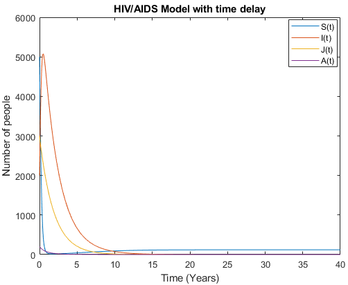
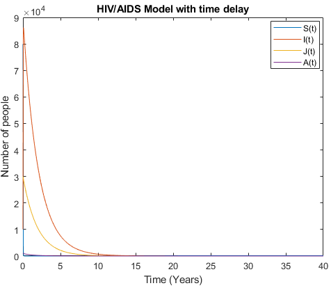
Mathematical analysis of model (3) is studied where \(R_{0}< 1\) with \(R_{0}= 0.3893\), the results show how disease disappear in middle ten to fifteen years due to treatment and isolation of people with AIDS cases as it is shown in Figure 4 and Figure 5.

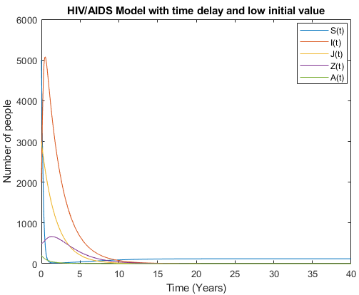
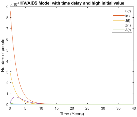
As the number of people who are un-aware about decrease, and a small number of people who tested negative who live in danger area to be infected with HIV is considered. The model (5) in Figures 6 and 7 show very accurate results compared to the model (3).

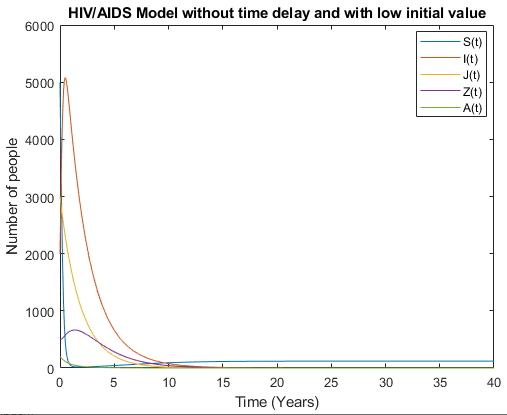
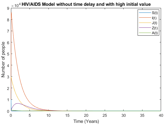
By accommodating pre-AIDS group with considering no time delay in Figures 8 and 9, the models behave almost the same as the number of people aware about their health status increase and the number of newborns who live with HIV decrease and tends to zero.

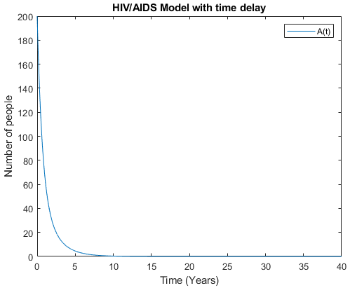
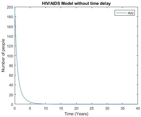
Let us compare each group by its own in model (5) with time delay and without time delay. Figures 10 and 11 show full AIDS group with time delay and without time delay respectively. Here, the model behaves almost the same as the number of people who are aware about their health status is big.

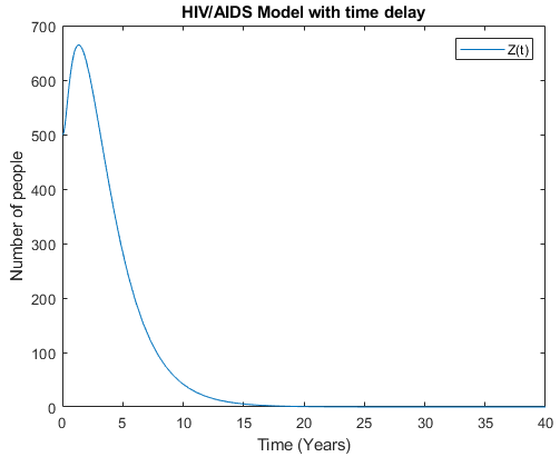
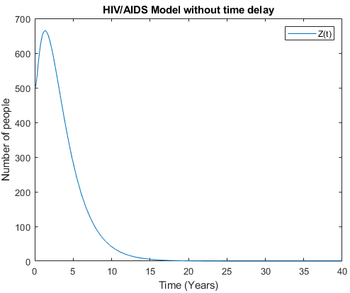
Figures 12 and 13 show Pre-AIDS group with time delay and without time delay respectively. These figures show that the model with time delay is doing better as people in Pre-AIDS group can live longer compared to those without time delay.

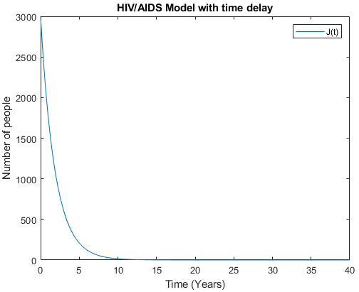
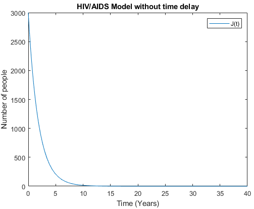
Figures 14 and 15 show the symptomatic group with time delay and without time delay respectively. The figures show that the model behaves almost the same as a high number of the symptomatic group is considered. As the number of people in the symptomatic group decrease and until they disappear, this implies the biggest reduction of number of people in full AIDS group.

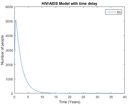
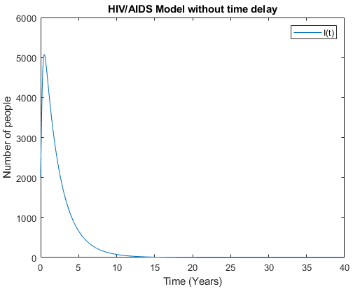
Figure 16 and 17 show the asymptomatic group with time delay and without time delay respectively. The figures show that the model behaves almost the same as a low number of asymptomatic group is considered. This also show that as the number of un-aware of their health status decreases, the number of people in Full AIDS group will decrease as well.

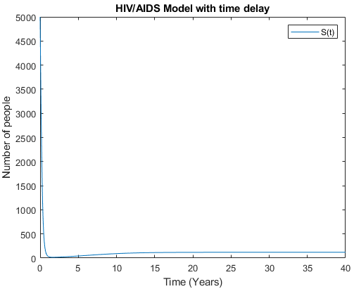
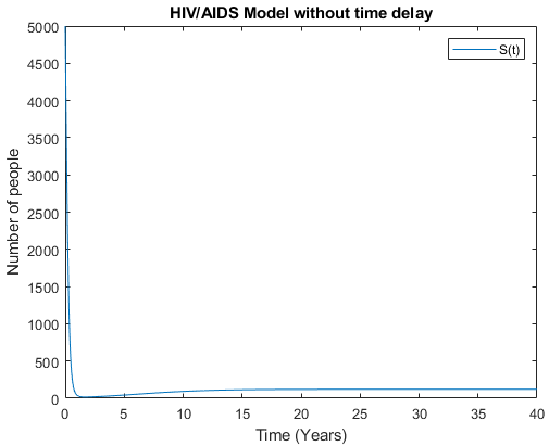
Figures 18 and 19 demonstrate the susceptible group with time delay and without time delay respectively. The figures show that the model behaves almost the same as the number of asymptomatic group decreases and symptomatic group increases. This shows that as the number of new infection decreases then the number of the susceptible group should increase.

5. Conclusion and recommendation

The HIV/AIDS model with treatment, time delay and vertical transmission is proposed in this study under some assumptions. We formulated a mathematical model diagram that involves five distinct sub-population groups. The basic reproduction number \(R_{0}\) has been calculated using the next generation matrix method. In addition, we determined the equilibrium points, i.e., disease free and endemic. The local and global stability of disease free and endemic are established. We also carried out numerical simulations of the stable states when \(R_0 < 1\). The study simulation results suggest a high number of people from symptomatic group (people aware of their health status) rather than isolating AIDS patients which is impossible in real life situation as these people serve society in various domains. As the number of symptomatic group is high, the risk of producing HIV-infected children become small and ignored in the model. Furthermore, the basic reproduction number \(R_{0}\) is computed and, due to the values of the parameters given, it is found that \(R_{0}=0.0011\) which is less than one, as this is an implication that the disease will disappear.

As limitation, authors didn't get real data to use in this study. Hence, parameters estimation were adopted. We therefore recommend further studies for HIV/AIDS infection predictions in 20, 50, 80, 100 years to come as the number of people living with HIV/AIDS is increasing with time according to literature.

Conflicts of Interest

The authors declare no conflict of interest.

References

1. Bellenir, K., & Dresser, P. D. (Eds.). (1996). Contagious and Non-contagious Infectious Diseases Sourcebook: Basic Information about Contagious Diseases Like Measles, Polio, Hepatitis B, and Infectious Mononucleosis, Non-contagious Infectious Diseases Like Tetanus and Toxic Shock Syndrome, and Diseases Occurring as Secondary Infections Such as Shingles and Reye Syndrome Along with Vaccination, Prevention, and Treament Information and a Section Describing Emerging Infectious Disease Threats (Vol. 8). Omnigraphics Incorporated. [Google Scholor]
2. Busenberg, S., & Cooke, K. (2012). Vertically Transmitted Diseases: Models and Dynamics(Vol. 23). Springer Science & Business Media. [Google Scholor]
3. Anderson, R. M., & May, R. M. (1992). Infectious Diseases of Humans: Dynamics and Control. Oxford University Press. [Google Scholor]
4. Hethcote, H. W., & Levin, S. A. (1989). Periodicity in Epidemiological Models. In Applied Mathematical Ecology (pp. 193-211). Springer, Berlin, Heidelberg. [Google Scholor]
5. Gottlieb, M. S., Schanker, H. M., Fan, P. T., Saxon, A., Weisman, J. D., & Pozalski, I. (1981). Pneumocystis pneumonia—Los Angeles. MMWR, 30(21), 250-252. [Google Scholor]
6. Cai, L., Li, X., Ghosh, M., & Guo, B. (2009). Stability analysis of an HIV/AIDS epidemic model with treatment. Journal of Computational and Applied Mathematics, 229(1), 313-323. [Google Scholor]
7. Report on the global AIDS Epidemic 2006. UNAIDS dWHO, 2006, UNAIDS/WHO New York.[Google Scholor]
8. Biswas, D., & Pal, S. (2017). Stability Analysis of a delayed HIV/AIDS Epidemic Model with Saturated Incidence. International Journal of Mathematics Trends and Technology, 43(3), 222-231. [Google Scholor]
9. Teng, T. R. Y., De Lara-Tuprio, E. P., & Macalalag, J. M. R. (2019, December). An HIV/AIDS epidemic model with media coverage, vertical transmission and time delays. In AIP Conference Proceedings (Vol. 2192, No. 1, p. 060021). AIP Publishing LLC. [Google Scholor]
10. Carvalho, A. R., Pinto, C. M., & Baleanu, D. (2018). HIV/HCV coinfection model: a fractional-order perspective for the effect of the HIV viral load. Advances in Difference Equations, 2018, Article No. 2, https://doi.org/10.1186/s13662-017-1456-z. [Google Scholor]
11. Krämer, A., Kretzschmar, M., & Krickeberg, K. (Eds.). (2010). Modern infectious disease epidemiology: Concepts, methods, mathematical models, and public health. Springer Science & Business Media. [Google Scholor]
12. Kou, C., Yan, Y., & Liu, J. (2009). Stability analysis for fractional differential equations and their applications in the models of HIV-1 infection. Computer Modeling in Engineering and Sciences (CMES), 39(3), 301. [Google Scholor]
13. Cai, L., Guo, S., & Wang, S. (2014). Analysis of an extended HIV/AIDS epidemic model with treatment. Applied Mathematics and Computation, 236, 621-627. [Google Scholor]
14. Stoddart, C. A., & Reyes, R. A. (2006). Models of HIV-1 disease: A review of current status. Drug Discovery Today: Disease Models, 3(1), 113-119. [Google Scholor]
15. Zafar, Z. U. A., Rehan, K., & Mushtaq, M. (2017). HIV/AIDS epidemic fractional-order model. Journal of Difference Equations and Applications, 23(7), 1298-1315. [Google Scholor]
16. Naik, P. A., Yavuz, M., & Zu, J. (2020). The role of prostitution on HIV transmission with memory: a modeling approach. Alexandria Engineering Journal, 59(4), 2513-2531. [Google Scholor]
17. Kribs-Zaleta, C. M., Lee, M., Román, C., Wiley, S., & Hernández-Suárez, C. M. (2005). The effect of the hiv/aids epidemic on africa's truck drivers. Mathematical Biosciences & Engineering, 2(4), 771. [Google Scholor]
18. Rao, A. S. S. (2003). Mathematical modelling of AIDS epidemic in India. Current Science, 84(9), 1192-1197. [Google Scholor]
19. Mukandavire, Z., Garira, W., & Chiyaka, C. (2007). Asymptotic properties of an HIV/AIDS model with a time delay. Journal of Mathematical Analysis and Applications, 330(2), 916-933. [Google Scholor]
20. Naresh, R., Tripathi, A., Tchuenche, J. M., & Sharma, D. (2009). Stability analysis of a time delayed SIR epidemic model with nonlinear incidence rate. Computers & Mathematics with Applications, 58(2), 348-359. [Google Scholor]
21. Osman, Z., & Abdurahman, X. (2015). Stability analysis of a delayed HIV/AIDS epidemic model with treatment and vertical transmission. Applied Mathematics, 6(10), 1781. [Google Scholor]
22. Naresh, R., Tripathi, A., & Omar, S. (2006). Modelling the spread of AIDS epidemic with vertical transmission. Applied Mathematics and Computation, 178(2), 262-272. [Google Scholor]
23. Li, M. Y., Smith, H. L., & Wang, L. (2001). Global dynamics of an SEIR epidemic model with vertical transmission. SIAM Journal on Applied Mathematics, 62(1), 58-69. [Google Scholor]
24. Naresh, R., & Sharma, D. (2011). An HIV/AIDS model with vertical transmission and time delay. World Journal of Modelling and Simulations, 7(3), 230-240. [Google Scholor]
25. Liu, J. L., & Zhang, T. L. (2012). Global stability for delay SIR epidemic model with vertical transmission. Open Journal of Applied Sciences, 2(4), 1-4. [Google Scholor]
26. Munawwaroh, D. A., Heri, R., Khabibah, S. U. S., & Anindita, H. P. (2020, April). Analysis stability of HIV/AIDS epidemic model of different infection stage in closed community. In Journal of Physics: Conference Series (Vol. 1524, No. 1, p. 012130). IOP Publishing. [Google Scholor]
27. HIV and its transmission. Centers for Disease Control and Prevention (CDC) and others. Divisions of HIV/AIDS Prevention, 2003. [Google Scholor]
28. AIDS statistics: 2019 Factsheet. UNAIDS. Global, HIV, 2019. [Google Scholor]
29. Bani-Yaghoub, M., Gautam, R., Shuai, Z., Van Den Driessche, P., & Ivanek, R. (2012). Reproduction numbers for infections with free-living pathogens growing in the environment. Journal of Biological Dynamics, 6(2), 923-940. [Google Scholor]
30. Yusuf, T. T., & Benyah, F. (2012). Optimal strategy for controlling the spread of HIV/AIDS disease: a case study of South Africa. Journal of Biological Dynamics, 6(2), 475-494. [Google Scholor]