On new approximations for the modified Bessel function of the second kind \(K_0(x)\)

1. Introduction

Recently, motivated by numerical problems raised by attempts to enhance the transmission rate of a particular communication system, which depends on modified Bessel functions of the second kind, \(K_\nu(x)\), a paper was published, based on novel approach, trying to rewrite those Bessel functions in series from using simple elementary functions [1]. However, no attention was given to the particular case of \(K_0(x)\) in this publication. Therefore, starting from the new series obtained in this paper for \(K_\nu(x)\), with \(\nu\neq 0\), we want to find out a series representation of the modified Bessel function of the second kind \(K_0(x)\) in terms of simple elementary functions (Section 2). The new approximation is analysed (Section 3) and then is compared with some well known series (Section 4). A new polynomial approximation is presented in Section 5 and final remarks are given in Section 6.

In [1], it is shown that, for \(\nu >0\), \(K_\nu(x)\) can be represented by an infinite series given by

with the coefficients where \(L(n,k)\) are the Lah numbers defined by with the conventions \(L(0,0) =1\), and \(L(n,0) = 0\), for \(n\geq 1\).

2. The case \(\nu =0\)

In order to get the expansion we are looking for, we start from the well known recursion formula [2] \[x K_{\nu-1}(x) - x K_{\nu+1}(x) = -2\nu K_{\nu}(x),\] which, from Equations (1-3) allow us to express \(K_0(x)\) as a sum of two series, i.e., where \(K_1 (x) = e^{-x} \displaystyle \sum_{n=0}^{\infty} \sum_{k=0}^{n} \, \Lambda(1,n,k)\, x^{k-1},\) and \(K_2 (x) = e^{-x} \displaystyle \sum_{n=0}^{\infty} \sum_{k=0}^{n} \, \Lambda(2,n,k)\, x^{k-2},\) with the respective coefficients \[\Lambda(1,n,k) = \frac{(-1)^k \, \sqrt{\pi}\, \Gamma(2)\, \Gamma \left(n- \frac{1}{2}\right) \, L(n,k)}{2^{1-k} \, \Gamma\left( -\frac{1}{2}\right) \, \Gamma \left( n+\frac{3}{2}\right)\, n!},\] and \[\Lambda(2,n,k) = \frac{(-1)^k\, \sqrt{\pi}\, \Gamma(4)\, \Gamma \left(n- \frac{3}{2}\right) \, L(n,k)}{2^{2-k} \, \Gamma\left( -\frac{3}{2}\right) \, \Gamma \left( n+\frac{5}{2}\right)\, n!}.\] The dependence of these coefficients on the \(\Gamma\) function can be removed by applying its recursion relations. Doing so, both coefficients can be written in a simpler formula as \[\Lambda(1,n,k) = \displaystyle \frac{(-1)^{k+1}}{2^{2-k}}\, \frac{1}{\left(n^2 -\frac{1}{4}\right)}\, \frac{L(n,k)}{n!},\] and \[\Lambda(2,n,k) = \displaystyle \frac{9}{2}\, \frac{(-1)^{k}}{2^{2-k}}\, \frac{1}{\left(n^2 -\frac{9}{4}\right) \,\left(n^2 -\frac{1}{4}\right)}\, \frac{L(n,k)}{n!}.\] Substituting these factors in Equation (4), we get, after a straightforward calculation, the polynomial expansion formula for \(K_0(x)\), namely Knowing that the confluent hypergeometric function (Kummer's function) of the first kind \({}_1F_1\) is given by \[{}_1F_1(1-n;2;2 x) = -\sum _{k=0}^n \frac{(n-1)!(-1)^k 2^{k-1} k\, x^{k-1}}{(k!)^2 (n-k)!} .\] The result of Equation (5) can be expressed in terms of only one summation of a well known function as or, more simply Recently, two finite sum representation formulae for the modified Bessel function of the second kind \(K_n(x)\) were established for positive integer order, one of them including \(K_0(x)\), \(K_1(x)\) and the generalized hypergeometric function \({}_1F_2\) [3].

3. Discussions of our result

We give the explicit values of the coefficients \(\Lambda(1,n,k)\), for \(n\) and \(k\) varying from 0 to 10 in Table 1. The coefficients \(\Lambda(2,n,k)\) can be straightforwardly obtained from the values of Table 1 by using the equality From Table 1 and from Equations (1) and (8), we can easily get the explicit formulae for a finite terms expansion of the Bessel functions for \(\nu =1\) and \(\nu =2\). Indeed, the truncated summation up to \(n=8\), for example, for \(K_1\) and \(K_2\) are, respectively, and

Table 1. Values for \(\Lambda(1,n,k)\).

n/k	\(k=0\)	\(k=1\)	\(k=2\)	\(k=3\)	\(k=4\)	\(k=5\)	\(k=6\)	\(k=7\)	\(k=8\)	\(k=9\)	\(k=10\)
0	1
1	0	2/3
2	0	2/15	-2/15
3	0	2/35	-4/35	4/105
4	0	2/63	-2/21	4/63	-2/189
5	0	2/99	-8/99	8/99	-8/297	4/1485
6	0	2/143	-10/143	40/429	-20/429	4/429	-4/6435
7	0	2/195	-4/65	4/39	-8/117	4/195	-8/2925	8/61425
8	0	2/255	-14/255	28/255	-14/153	28/765	-28/3825	8/11475	-2/80325
9	0	2/323	-16/323	112/969	-112/969	56/969	-224/14535	32/14535	-16/101745	4/915705
10	0	2/399	-6/133	16/133	-8/57	8/95	-8/285	32/5985	-8/13965	4/125685	-4/5655825

Table 2. Values for \(K_0 (x)\) expansion given by Equation (5) for different \(n\) values.

x	\(K_0(x)\)	\(K_0(x)\) expansion up to n
		1.72407	1.63	1.7402	0.71	1.75031	0.14
0.3	1.37246	1.35125	1.55	1.37292	0.03	1.37533	0.21
0.4	1.11453	1.10552	0.81	1.1174	0.26	1.11603	0.13
0.5	0.924419	0.922763	0.18	0.926341	0.21	0.924409	0.0011
0.6	0.777522	0.779281	0.23	0.778119	0.076	0.776932	0.076
0.7	0.66052	0.663358	0.43	0.66026	0.039	0.659982	0.081
0.8	0.565347	0.568067	0.48	0.564752	0.11	0.56509	0.045
0.9	0.48673	0.488824	0.43	0.48615	0.12	0.486736	0.0012
1.0	0.421024	0.422366	0.32	0.420628	0.094	0.421182	0.037
5.0	\(3.69\times10^{-3}\)	\(3.66\times10^{-3}\)	1.03	\(3.69\times10^{-3}\)	0.10	\(3.69\times10^{-3}\)	0.08

From Equations (9) and (10), the well known curves for both Bessel functions are reproduced with accuracy.

We can now plot the function given by Equation (5). All plots in this paper were made by using the software Mathematica, version 12.1.

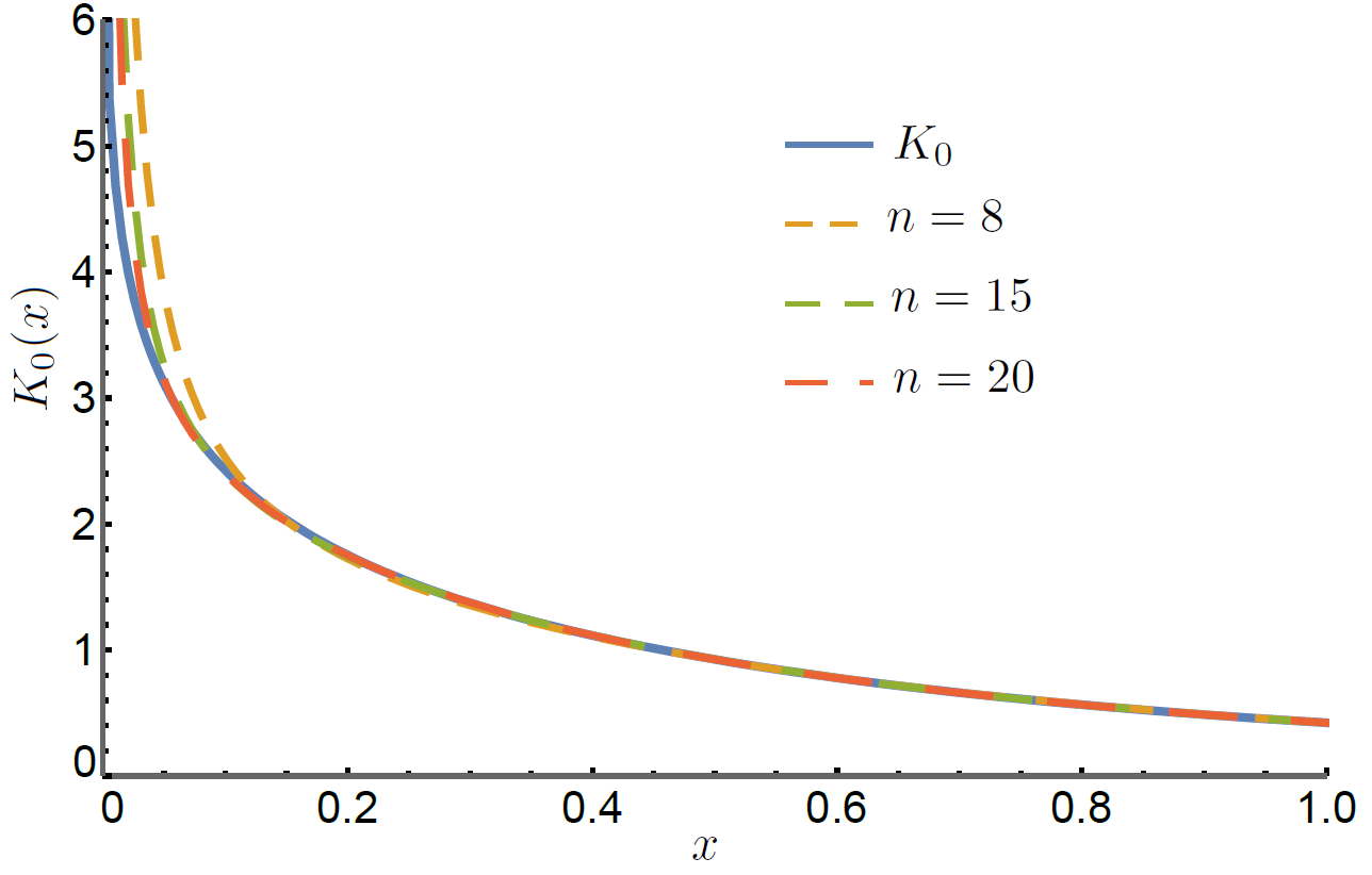
In Figure 1, three approximation functions for \(K_0(x)\), each with a different number of terms, \(n\), are compared with the well known behavior of \(K_0(x)\) without any approximation.

We can easily see that the result is not so good for \(x \lesssim 0.1\).

Some particular values for \(K_0(x)\) are given in Table 2, for the interval \(0.1 \leq x \leq 5.0\) where the relative error \(|\epsilon_r|\) is defined by

\[|\epsilon_r| =\displaystyle\frac{ \left|K_0(x) - K_0(x)\big|_{\text{approx}}\right|}{K_0}.\] Notice that the maximum value of \(|\epsilon_r|\), in this interval, corresponding to the cases \(n=15\) and \(n=20\), is of the order of 1%.

For the expansion of \(K_0(x)\) up to \(n=8\), we have a relative error of \(\simeq 4%\) for \(x=0.1\) (See Table 2). However, we get an error of \(10%\) or more when \(x \leq 0.0741\). For \(n=15\), the error is \(\simeq 1%\) or less, when \(0.0676 \leq x \leq 7\), and an error of \(10%\) or more when \(x \leq 0.0376\). Finally, for \(n=20\), we have an error of \(1%\) or less when \(0.0505 \leq x \leq 7.8\) and an error of \(10%\) or more when \(x \leq 0.0274\).

Table 3. Values for \(K_1(x)\) and \(K_2(x)\) obtained from Equations (9) and (10) up to \(n=8\). The error here is the difference between the value found and the expected value.

\(x\)	\(K_1(x)\)	\(K_2(x)\)
0.05	19.892 \(\pm\) 0.0176934	799.514 \(\pm\) 0.0125116
0.1	9.84899 \(\pm\) 0.00485623	199.507 \(\pm\) 0.00260945
0.5	1.65683 \(\pm\) 0.000392678	7.55012 \(\pm\) 0.000066483
1.0	0.601256 \(\pm\) 0.000650892	1.62492 \(\pm\) 0.0000855086
5.0	0.00413672 \(\pm\) 0.0000921043	0.0053286 \(\pm\) 0.0000196572
10.0	0.000080361 \(\pm\) 0.0000617122	0.000021682 \(\pm\) 1.72217\(\times10^{-7}\)

In order to understand why the expansion for \(K_1(x)\) and \(K_2(x)\) have a great fit even for small values of \(x\) but \(K_0(x)\) shows a much larger error for the same small \(x\) values we have to look carefully at Equation (5). The problem is that the first term of Equation (5) is the division \(K_1(x)/x\). Therefore, for very small values of \(x\), the error in the series predictions for \(K_1(x)\) is amplified.

In Table 3, some values of \(K_1(x)\) and \(K_2(x)\) are shown with the respective absolute error, for the interval \(0.05 \leq x \leq 10\).

So, while the absolute errors in \(K_1(0.05)\) and \(K_2(0.05)\) are of the order of \(10^{-2}\), the error found for \(K_0(0.05)\), given by Equation (5), is \(\simeq0.35\), which is an order of magnitude greater than the error just in \(K_1(0.05)\). The situation tends to become worse when \(x \rightarrow 0\).

4. Comparison with other series

Let us now compare our approximation for \(K_0(x)\) with others found in the literature. The first one is given in Watson's book [2]: in which \(\psi(n) = \displaystyle -\gamma + \sum_{k=1}^{n-1} k^{-1} \ \ (n \geq 2)\), where \(\gamma\) is the Euler constant.

The second approximation is given by Equation 9.6.54 of [4]

The next two are valid only for specific domains. Equation 9.8.5 of [4], for example, is valid for the interval \(0< x\leq 2\): with \(|\epsilon| < 1\times 10^{-8}\).

Starting from equation 5.39 of Bowman's book [5], we get Equation 9.8.6 of [4], which is valid for the interval \(2\leq x < \infty\):

where \(|\epsilon| < 1.9\times 10^{-7}\).

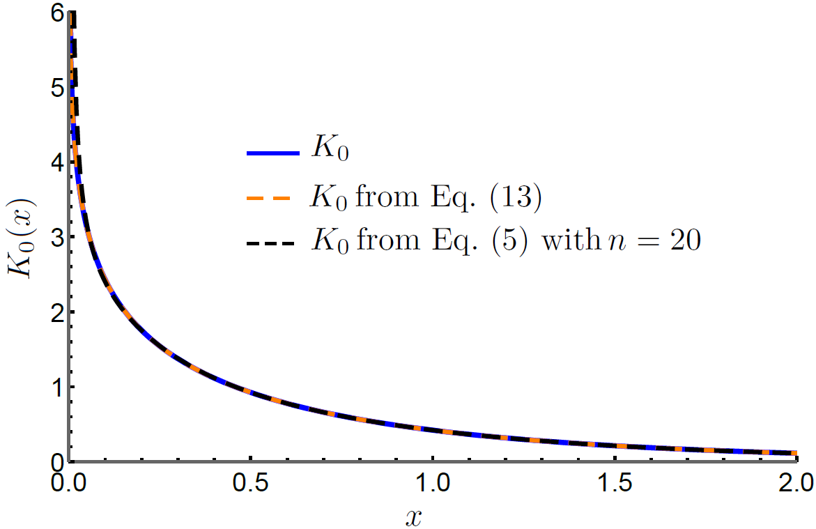
In order to check the accuracy of our result, Equation (5) or (6), let's first compare it graphically with Equations (13) and (14), which are the two approximations with the lowest errors. The comparison is made in Figures 2 and 3, respectively for the intervals \(0< x\leq 2\) and \(2\leq x< 10\).

5. Improving the polynomial approximation

In spit of the qualitative agreement graphically obtained, the error values displayed in Table 2 show that the approximation given by Equation (5) or (6) is far from being the best choice. This unexpected result motivates us now to try to improve the approximations given by Equations (13) and (14). This was done by fitting the Bessel function \(K_0(x)\) by a similar polynomials using the Software Mathematica. For this, we still maintain the two distinct regions \(0< x \leq 2\) and \(2 \leq x < \infty\).

Using Equation (13) as a starting point, and keeping the polynomial order, we find, for \(0< x\leq 2\), the following new expression:

From Equation (14), at the same interval \(2\leq x< \infty\), we get the following result: In Table 4, we compare the relative errors of Equations (15) and (16) with those of the Equations (13) and (14) which generalize them.

Table 4. This Table shows the approximations' errors, taking into account those of Abramowitz's Handbook, Equations~(\ref{9-8-5}) and (\ref{9-8-6}), and comparing them, respectively, to the analogous new polynomial approximation we propose, given by Equations~(\ref{9-8-5-2}) and (\ref{9-8-6-2}).

0.05	\(1.54698\times 10^{-7}\)	\(2.19076\times 10^{-10}\)	--	--
0.1	\(1.88413\times 10^{-7}\)	\(2.25679\times 10^{-10}\)	--	--
0.5	\(9.43814\times 10^{-8}\)	\(6.78598\times 10^{-10}\)	--	--
1.0	\(8.17407\times 10^{-7}\)	\(4.93335\times 10^{-10}\)	--	--
2.0	\(6.36598\times 10^{-6}\)	\(3.03931\times 10^{-8}\)	\(2.86954\times 10^{-7}\)	\(2.43697\times 10^{-14}\)
5.0	--	--	\(1.2982\times 10^{-6}\)	\(2.55901\times 10^{-11}\)
10.0	--	--	\(2.15433\times 10^{-6}\)	\(1.39165\times 10^{-7}\)
15.0	--	--	\(4.37274\times 10^{-6}\)	\(3.94849\times 10^{-6}\)
20.0	--	--	\(9.60195\times 10^{-6}\)	\(1.10755\times 10^{-5}\)

An inspection of Table 4 shows first that, in the range \(0 < x \leq 2\), our result is almost \(10^3\) times more accurate than that of Equation (13). For the second range, the relative errors associated to our new results are much better than the other. In particular, the error is \(10^7\) times smaller for \(x=2\), \(10^5\), when \(x=5\), and of the same order of magnitude elsewhere.

6. Conclusion

We got a series representation for the Bessel function \(K_0(x)\) in terms of confluent hypergeometric functions, and two polynomial approximations for the same function. It is shown that expressions based on a certain number of terms (\(n=8, 15\) and \(20\)) of the infinite series are not more accurate than few other approximations found in the literature. However, the two new polynomial approximations proposed are orders of magnitude more accurate than the standard approximation found in the Abramowitz and Stegun's Handbook.

Acknowledgments

One of us (FS) was financed in part by the Coordenação de Aperfeiçoamento de Pessoal de Nível Superior - Brazil (CAPES), Finance Code 001. We are grateful to an anonymous referee for his criticism and fruitful comments.

Author Contributions

All authors contributed equally to the writing of this paper. All authors read and approved the final manuscript.

Conflicts of interest

The authors declare no conflict of interest.

References

Molu, M. M., Xiao, P., Khalily, M., Zhang, L.,& Tafazolli, R. (2017). A novel equivalent definition of modified Bessel functions for performance analysis of multi-hop wireless communication systems. IEEE Access, 5, 7594-7605.[Google Scholor]
Watson, G. N. (1966). A Treatise on the Theory of Bessel Functions, 2nd Edition. Cambridge University Press, London. [Google Scholor]
Maširevic, D. J., & Pogány, T. K. (2019). On series representations for modified Bessel function of second kind of integer order. Integral Transforms and Special Functions, 30(3), 181-189.
[Google Scholor]
Abramowitz, M., & Stegun, I. A. (1970). Handbook of Mathematical Functions with Formulas, Graphs and Mathematical Tables. Dover Publications, New York. [Google Scholor]
Bowman, F. (2010). Introduction to Bessel Functions. Dover Publications, New York. [Google Scholor]