
Dealing with the complexities of bounded variables measuring certain characteristics of phenomenon is common in many areas of applied science. In particular, in psychology, economics, and biology, variables like proportions of a particular attribute, scores on various aptitude tests, multiple indices, and rates set on the interval \( (0, 1) \) are often encountered. Continuous probability distributions with support of \((0, 1)\), known as unit distributions, are required for an adequat modeling of these variables. The most widely used two-parameter unit distribution is the beta distribution (see [1]). When fitting data with a physical maximum, the beta distribution works great, but has some limitations in the other cases. The recent rise in the number of research papers devoted to the development of new unit interval distributions demonstrates their growing importance. Table 1 provides a quick overview of other unit distributions that have been proposed as alternatives to the beta distribution.
These distributions are dependent on one or more parameters. Their key functions have specific characteristics that are desirable in some statistical modeling context dealing with data over the interval \((0, 1)\). The majority of the recent distributions in Table 1 are created using a suitable variable transformation of a positive support baseline distribution. The main popular transformations are ratio-polynomial or exponential functions, such as \(l(x)=x/(1+x)\), \(l(x)=1/(1+x)\), or \(l(x)=e^{-x}\). Some other unit distributions are based on original analytical definitions, such as the Power (Po) distribution defined with the following cumulative distribution function (cdf):
| Common name | Reference |
|---|---|
| Johnson \({S_B}\) | [2] |
| Topp-Leone | [3] |
| unit gamma | [4] |
| Kumaraswamy | [5] |
| standard two-sided power | [6] |
| log-Lindley | [7] |
| unit Weibull | [8, 9] |
| unit Birnbaum-Saunders | [10] |
| unit Gompertz | [11] |
| log-xgamma | [12] |
| unit inverse Gaussian | [13] |
| logit slash | [14] |
| unit generalized half normal | [15] |
| \(2^{nd}\) degree unit Lindley | [16] |
| unit Johnson SU | [17] |
| log-weighted exponential | [18] |
| unit Rayleigh | [19] |
| unit modified Burr-III | [20] |
| arcsecant hyperbolic normal | [21] |
| unit Burr-XII | [22] |
| unit power-logarithmic | [23] |
| transmuted unit Rayleigh | [24] |
| trapezoidal beta | [25] |
| unit half-normal distribution | [26] |
For the case of \(\alpha>0\), the UPL distribution was introduced and studied in-depth in [23]. For \(\alpha>0\), the properties of this distribution are as follows: (a) its pdf is defined as an original power-logarithmic scheme which is inspired by the famous Box-Cox transformation, (b) this function is increasing and can be highly asymmetric on the left, with various types of angular and J forms, which is a relatively uncommon property for a one-parameter unit distribution, (c) it has solid results in stochastic orders showing some relationship with the Po distribution, (d) its hazard rate function (hrf) is increasing, (e) simple expressions exist for a variety of moments-related quantities, such as ordinary moments, moment generating function, incomplete moments, logarithmic and logarithmically weighted moments, (f) the behavior of the moments skewness and kurtosis of the distribution is very manageable, and (g) it has a wide range of applications and can be used to build new statistical models as a generator. Despite these originalities, the main drawback of the UPL distribution is that the cdf is only defined with special integral functions; it has not a simple analytical expression. In particular, it is an obstacle for the in-depth quantile analysis of the distribution.
In this article, we contribute to the development of the power-logarithmic scheme to develop a new one-parameter unit distribution with interesting features. More precisely, we apply the power-logarithmic scheme to construct a valid cdf, instead of a power-logarithmic pdf as in the UPL distribution. As a result, the proposed distribution stands from the others by satisfying the following combined properties: (a) it is based on a single positive parameter, (b) its cdf presents various convex and concave shapes, (b) its pdf can be decreasing or U shaped, which is a relatively uncommon property for a unit distribution, (c) it has proven to be effective in stochastic orders, showing some relationship with the Po distribution, (d) it has a manageable quantile function (qf) based on the well-known Lambert function (principal branch), (e) its hrf has various types of U shapes, (f) simple expressions exist for a variety of moments-related quantities, such as ordinary moments, moment generating function, and incomplete moments, (g) the behavior of the moments skewness and kurtosis of the distribution is understable, and (h) it can perform better than the UPL and Po distributions in the context of data fitting. All these aspects are developed through mathematical, numerical and graphical investigations. We thus put the basics on a new one-parameter unit distribution that could serve in the future for various statistical objectives. As complementary results, we use the new distribution to determine some integrals linked to the Euler constant, which seem to not have received attention in the literature.
The following is the plan of the rest of the article. The new unit distribution is defined in Section 2, with analytical and graphical studies of its key functions. Section 3 is dedicated to some properties, such as diverse first order stochastic dominance, quantile analysis, and distributional results. A moment analysis is performed in Section 4. Section 5 provides some statistical perspectives of the new distribution. Complementary integral result are given in Section 6. Section 7 brings the article to a close.
Proposition 1. Let \(\alpha>0\). Then, the following ratio function has the properties of a continuous cdf: \begin{align*} F_{\alpha}(x)=\begin{cases}\displaystyle \frac{x^{\alpha}-1}{\alpha\log(x)} &\text{for}\ \ x\in (0,1),\\ 0 &\text{for}\ \ x\le 0,\\ 1& \text{for}\ \ x\ge 1.\end{cases} \end{align*}
Proof. By using standard asymptotic arguments, we have
\begin{align*}F_{\alpha}(x)&\underset{x\rightarrow 0}{\sim}-\frac{1}{\alpha \log(x)}\rightarrow 0,\\ F_{\alpha}(x)&=\frac{e^{\alpha \log(x)}-1}{\alpha\log(x)}\underset{x\rightarrow 1}{\sim} \frac{\alpha \log(x)}{\alpha \log(x)}=1.\end{align*} The function \(F_{\alpha}(x)\) is continuous for any \(x\in\mathbb{R}\). For any \(x\in (0,1)\), we have \begin{align*} F^{\prime}_{\alpha}(x)=\frac{\alpha x^{\alpha}\log(x)+1-x^{\alpha}}{\alpha x (\log(x))^2}. \end{align*} Owing to the following logarithmic inequality: \(\log(1+y)> y/(1+y)\), with \(y\in (-1,0)\), since \(y=x^{\alpha}-1 \in (-1,0)\) for \(x\in (0,1)\), we obtain \(\alpha \log(x)=\log(x^{\alpha})>1-1/x^{\alpha}\) which entails that \(\alpha x^{\alpha}\log(x)+1-x^{\alpha}> 0\) for \(x\in (0,1)\). Since the denominator is obviously positive too, we have \(F^{\prime}_{\alpha}(x)>0\) for any \(x\in (0,1)\), implying that \(F_{\alpha}(x)\) is strictly increasing on this interval. Therefore, \(F_{\alpha}(x)\) is increasing for \(x\in\mathbb{R}\). The proof of Proposition 1 is now complete.Thus, the cdf described in Proposition 1 defines a unit distribution, that we call the ratio power-logarithmic (RPL) distribution. When the parameter needs to be accurate, we refer to it as RPL\((\alpha)\) distribution. Even though it has a relationship with the UPL distribution, it is new to our knowledge in the literature. Indeed, one can remark that \(F_{\alpha} (x)\) is related to the pdf of the UPL distribution by the following equation:
The first notable properties of the cdf \(F_{\alpha}(x)\) are developed below.
Proposition 2. The cdf \(F_{\alpha}(x)\) is decreasing with respect to \(\alpha\), and, for any \(x\in (0,1)\), \(F_{\alpha}(x) \underset{\alpha\rightarrow 0}{=}1\) and \(F_{\alpha}(x) \underset{\alpha\rightarrow +\infty}{=}0\).
Proof. For \(x\in (0,1)\), we have
\begin{align*} \frac{\partial}{\partial \alpha}F_{\alpha}(x)=\frac{\alpha x^{\alpha}\log(x)+1-x^{\alpha}}{\alpha^2 \log(x)}=\frac{x\log(x)}{\alpha}F^{\prime}_{\alpha}(x). \end{align*} Therefore, since \(F^{\prime}_{\alpha}(x)>0\) and \(x\log(x)/\alpha< 0\), we have \(\partial F_{\alpha}(x)/\partial \alpha< 0\), and \(F_{\alpha}(x)\) is strictly decreasing with respect to \(\alpha\) for \(x\in (0,1)\), and just decreasing for \(x\in \mathbb{R}\). Furthermore, by using standard asymptotic arguments, we have \[F_{\alpha}(x)=\frac{e^{\alpha\log(x)}-1}{\alpha\log(x)}\underset{\alpha\rightarrow 0}{\sim}\frac{\alpha \log(x)}{\alpha \log(x)}=1,\] and, more directly, \[F_{\alpha}(x)\underset{\alpha\rightarrow +\infty}{\sim}-\frac{1}{\alpha\log(x)}\underset{\alpha\rightarrow +\infty}{=}0.\] The stated results are obtained.These properties are illustrated in Figure 1.
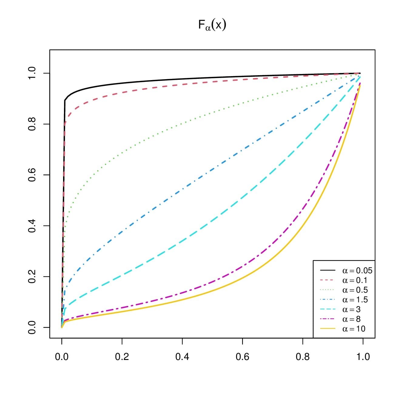
The various convex and concave shapes of \(F_{\alpha}(x)\) demonstrate the great modeling capacities of the RPL distribution.
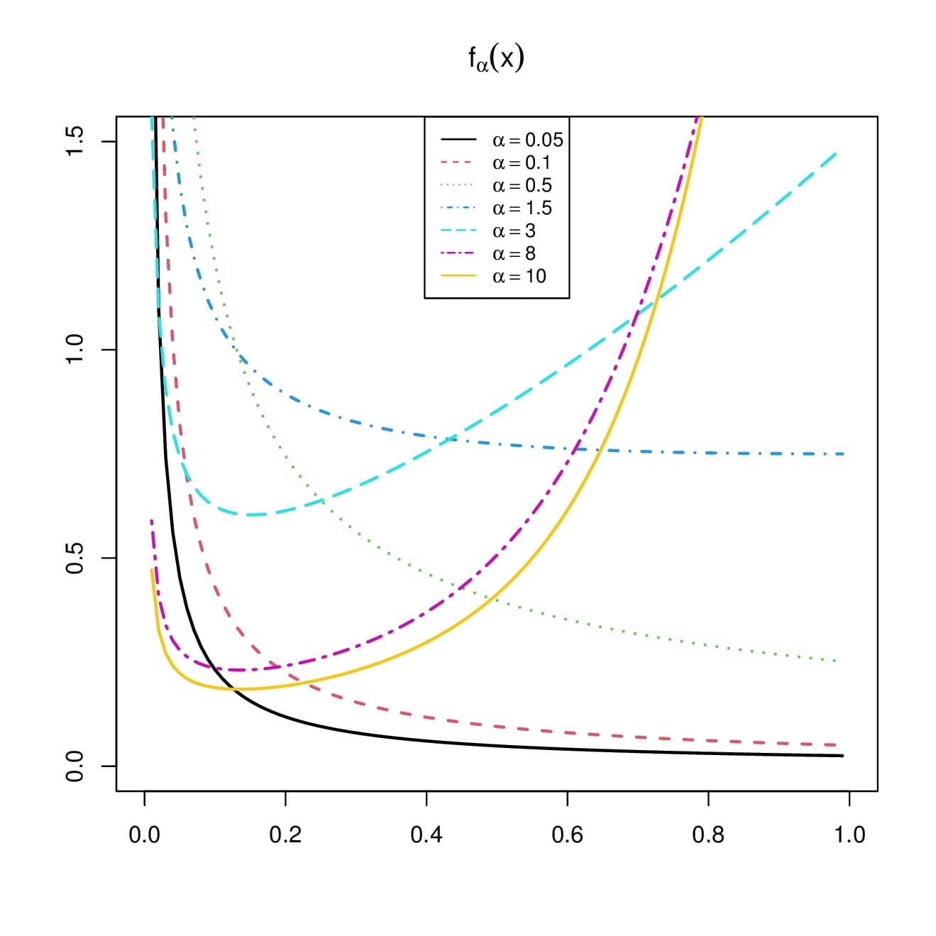
From Figure 2, we see that the pdf of the RPL distribution can be decreasing for the small values of \(\alpha\), or U shapes.
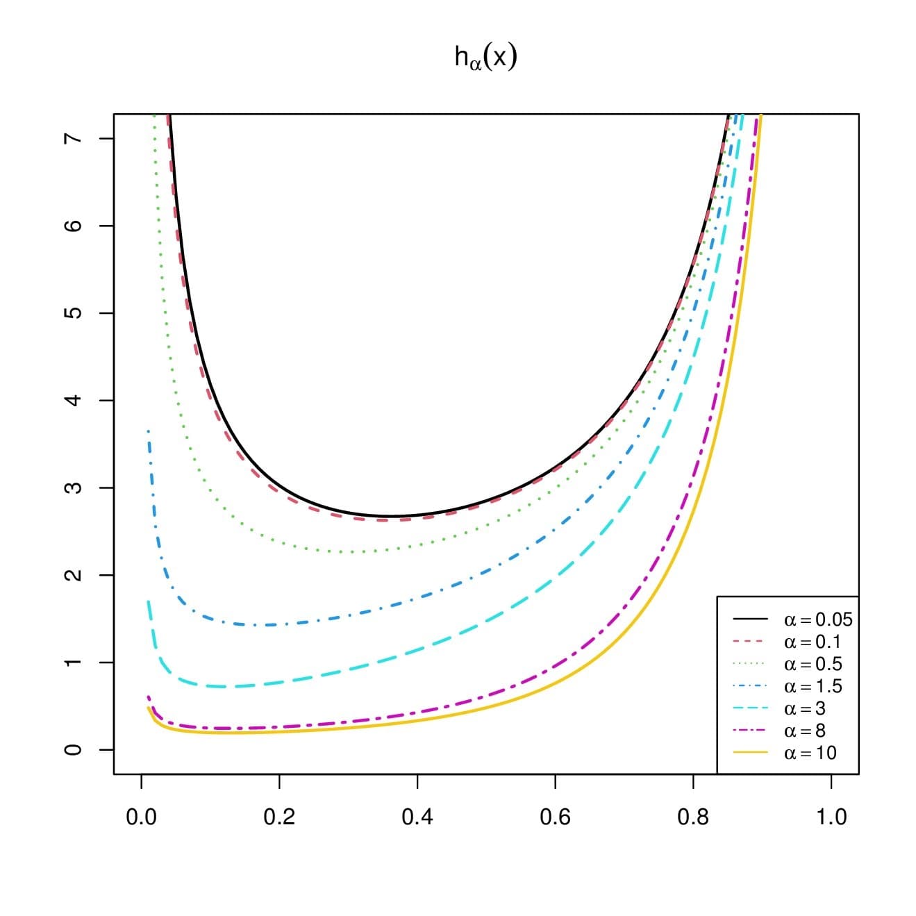
A brief study of \(h_{\alpha}(x)\) is now provided. At the boundaries, the following results hold:
\[h_{\alpha}(x)\underset{x\rightarrow 0}{\sim} \frac{1}{\alpha x (\log(x))^2} \rightarrow +\infty, \quad h_{\alpha}(x) \underset{x\rightarrow 1}{\sim} \frac{1}{1-x}\rightarrow +\infty.\] The precise analytical behavior of \(h_{\alpha}(x)\) is difficult to analyse; its derivative is very sophisticated. As a result, we conduct a graphical analysis to comprehend its shape behavior. Figure 3 depicts some curves of \(h_{\alpha}(x)\) for various values of \(\alpha \). It is clear from Figure 3 that the hrf of the RPL distribution is exclusively U shaped.Proposition 3. The following first order stochastic dominance results hold:
Proof. Let us prove the two results in turns.
Proposition 4. The qf of the RPL distribution is expressed as \[Q_{\alpha}(u)=\left[-u W_{0}\left( -\frac{1}{u} e^{-1/u}\right) \right]^{1/\alpha}, \quad u\in (0,1),\] where \(W_{0}(x)\) denotes the principal branch of the Lambert function.
Proof. By its definition, the qf is \(Q_{\alpha}(u)=F^{-1}_{\alpha}(u)\) and hence satisfies the following equation: \(F_{\alpha}(y)=u\) according to \(y\). With step by step development, we obtain
\( u =F_{\alpha}(y)\ \Leftrightarrow \ u = \frac{y^{\alpha}-1}{\alpha\log(y)} \ \Leftrightarrow \ \log(y^{\alpha}) = \frac{y^{\alpha}}{u}-\frac{1}{u}\ \Leftrightarrow \ y^{\alpha}= e^{y^{\alpha}/u}e^{-1/u} \ \Leftrightarrow \ -\frac{y^{\alpha}}{u} e^{-y^{\alpha}/u}=-\frac{1}{u} e^{-1/u} \ \Leftrightarrow \ -\frac{y^{\alpha}}{u} = W_{0}\left( -\frac{1}{u} e^{-1/u}\right)\ \Leftrightarrow \ y=\left[-u W_{0}\left( -\frac{1}{u} e^{-1/u}\right) \right]^{1/\alpha}. \)The stated expression is obtained.
The next proposition is about the behavior of the qf with respect to the parameter \(\alpha\).Proposition 5. The qf \(Q_{\alpha}(u)\) is strictly increasing with respect to \(\alpha\) for \(u \in (0,1)\), and \[Q_{\alpha}(u) \underset{\alpha\rightarrow 0}{=}0, \quad Q_{\alpha}(u) \underset{\alpha\rightarrow +\infty}{=}1.\]
Proof. First, since \(Q_{\alpha}(u)\in (0,1)\) for any \(u\in (0,1)\), we have \begin{align*} \frac{\partial}{\partial \alpha}Q_{\alpha}(u)& =\frac{\partial}{\partial \alpha}e^{(1/\alpha)\log \left[-u W_{0}\left( – e^{-1/u}/u\right) \right]}\\ & =-\frac{1}{\alpha^2} \log \left[-u W_{0}\left( -\frac{1}{u} e^{-1/u}\right) \right] e^{(1/\alpha)\log \left[-u W_{0}\left( – e^{-1/u}/u\right) \right]}\\ & = -\frac{1}{\alpha} \log(Q_{\alpha}(u) ) Q_{\alpha}(u)>0. \end{align*} Therefore, \(Q_{\alpha}(u)\) is a strictly increasing function with respect to \(\alpha\) for \(u\in (0,1)\). The values of the limits are derived from the following expression: \(Q_{\alpha}(u)=v^{1/\alpha}\) with \(v=-u W_{0}\left( -e^{-1/u}/u\right) \in (0,1) \) independent of \(\alpha\); we have \(Q_{\alpha}(u) \underset{\alpha\rightarrow 0}{=}0\) and \(Q_{\alpha}(u) \underset{\alpha\rightarrow +\infty}{=}v^0=1\). Proposition 5 is proved.
It is worth noting that the Lambert function is implemented in the majority of mathematical software, allowing the study of \(Q_{\alpha}(u)\). With the help of the library lawW of the R software (see [29]), Figure 4 depicts some curves of \(Q_{\alpha}(u)\) for several values of \(\alpha\).
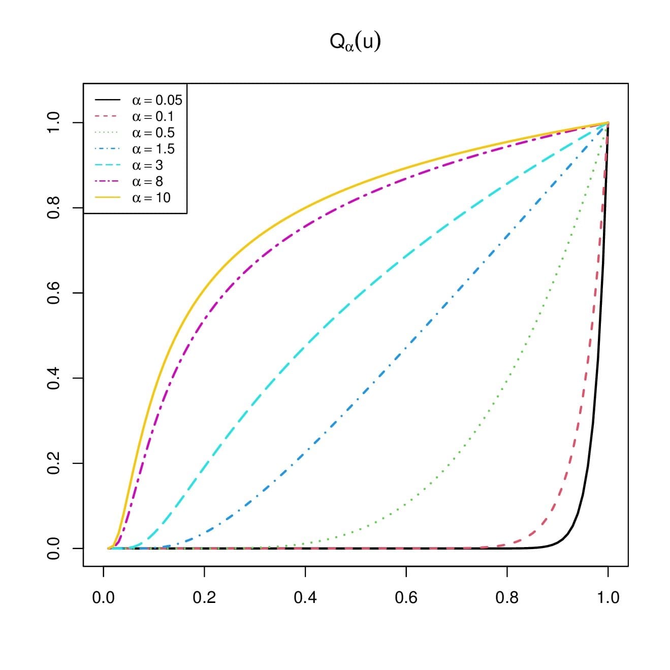
We notice a large panel of convex and concave shapes, revealing a certain level of quantile flexibility. In addition, a clear hierarchy of the curves can be seen for increasing values of \(\alpha\), ilustrating the results in Proposition 5.
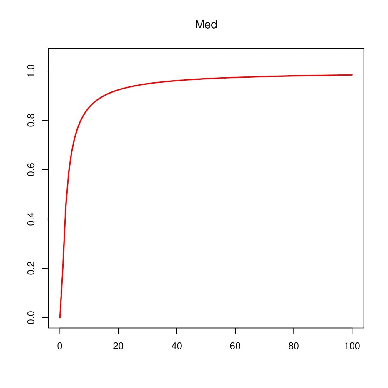
On the other hand, Proposition 5 implies that the median defined by Med\(=Q_{\alpha}(1/2)\) is an increasing function with respect to \(\alpha\). This fact is illustrated in Figure 5.
A more in-depth quantile analysis of the RPL distribution, including the expressions of the quantile density function, hazard quantile function, quantile asymmetry and plateness measures, is possible thanks to Proposition 4. In survival studies, [30] and [31] demonstrate the importance of these quantities.
Proposition 6. Let \(X\) be a random variable with the RPL\((\alpha)\) distribution and \(r\) be a positive integer. Then, the \(r\)th ordinary moment of \(X\) is obtained as \begin{align*} m_{\alpha}(r)=\mathbb{E}(X^r)=1 – \frac{r}{\alpha}\log\left(1+\frac{\alpha}{r}\right). \end{align*} The case \(r=0\) is not covered by this formula, but we can set \(m_{\alpha}(0)=\mathbb{E}(X^0)=1\).
Proof. Through the integral definition of the \(r\)th ordinary moment, we have \[m_{\alpha}(r)=\int_{-\infty}^{+\infty}x^r f_{\alpha}(x)dx=\frac{1}{\alpha}\int_{0}^{1}x^{r-1} \frac{\alpha x^{\alpha}\log(x)+1-x^{\alpha}}{(\log(x))^2} dx.\] Let us now introduce the following function of \(\alpha\): \begin{align*} \Psi_{r}(\alpha)&=\int_{0}^{1}x^{r-1} \frac{\alpha x^{\alpha}\log(x)+1-x^{\alpha}}{(\log(x))^2} dx, \end{align*} with \(\Psi_{r}(\alpha)=0\) for \(\alpha=0\). By applying the Leibnitz integral rule, we get \begin{align*} \frac{\partial}{\partial \alpha}\Psi_{r}(\alpha)&= \frac{\partial}{\partial \alpha}\int_{0}^{1}x^{r-1} \frac{\alpha x^{\alpha}\log(x)+1-x^{\alpha}}{(\log(x))^2} dx =\int_{0}^{1}x^{r-1} \frac{1}{(\log(x))^2}\frac{\partial}{\partial \alpha} (\alpha x^{\alpha}\log(x)+1-x^{\alpha}) dx\\ & = \int_{0}^{1}x^{r-1}\frac{1}{(\log(x))^2} \times \alpha x^{\alpha } (\log(x))^2dx= \alpha \int_{0}^{1}x^{r+\alpha-1}dx=\frac{\alpha}{r+\alpha}=1- \frac{r}{r+\alpha}. \end{align*} Upon integrating with respect to \(\alpha\), we obtain \(\Psi_{r}(\alpha)=\alpha – r\log(r+\alpha)+c\), where \(c\) denotes a generic constant at this step. Since \(\Psi_{r}(0)=0\), we have \(c=r\log(r)\). Therefore \[\Psi_{r}(\alpha)=\alpha – r\log(r+\alpha)+r\log(r)=\alpha – r\log\left(1+\frac{\alpha}{r}\right).\] Hence \[m_{\alpha}(r)=\frac{1}{\alpha}\Psi_{r}(\alpha)=1 – \frac{r}{\alpha}\log\left(1+\frac{\alpha}{r}\right),\] ending the proof of Proposition 6.
Some properties of the ordinary moments are expressed in the next result.
Proposition 7. The following properties of the ordinary moments hold:
Proof.
This ends the proof of Proposition 7.
We now illustrate the findings of Proposition 7 in Figure 6, by plotting \(m_r(\alpha)\) for various values of \(r\) and \(\alpha\).
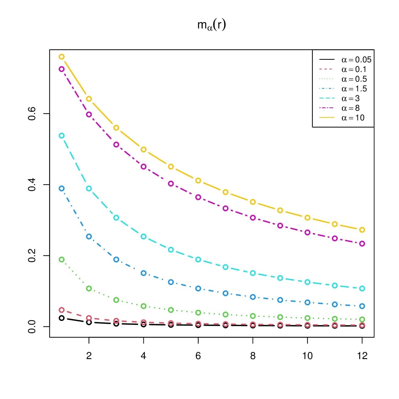
From this figure, we clearly see that \(m_{\alpha}(r)\) is a strictly increasing function with respect to \(\alpha\), and a strictly decreasing function with respect to \(r\).
Based on Proposition 6, the mean of \(X\) is given as
\[m_{\alpha}=m_{\alpha}(1)=\mathbb{E}(X)=1 – \frac{1}{\alpha}\log\left(1+\alpha\right)\] and the variance of \(X\) is obtained as \begin{align*} \sigma_{\alpha}^2& = \mathbb{V}(X)=m_{\alpha}(2)-m_{\alpha}(1)^2=1 – \frac{2}{\alpha}\log\left(1+\frac{\alpha}{2}\right) – m_{\alpha}^2\\ & =\frac{1}{\alpha^2}\left[ 2\alpha \log(1+\alpha)-\log(1+\alpha)^2-2\alpha \log\left(1+\frac{\alpha}{2}\right) \right]. \end{align*} Also, the skewness and kurtosis coefficients of \(X\) are given as \begin{align*} \gamma_{\alpha}=\frac{m_{\alpha}(3)-3m_{\alpha} \sigma_{\alpha}^2-m_{\alpha}^3}{\sigma_{\alpha}^3}, \quad \beta_{\alpha}=\frac{m_{\alpha}(4)-4m_{\alpha}(3) m_{\alpha}+6m_{\alpha}(2) m_{\alpha}^2-3 m_{\alpha}^4}{\sigma_{\alpha}^4}, \end{align*}respectively. In our context, \(\gamma_{\alpha}\) is a measure of relative symmetry, and \(\beta_{\alpha}\) is a measure of the relative peakedness of the RPL distribution. Figure 7 presents the curves for \(\gamma_{\alpha}\) and \(\beta_{\alpha}\) with respect to \(\alpha\).
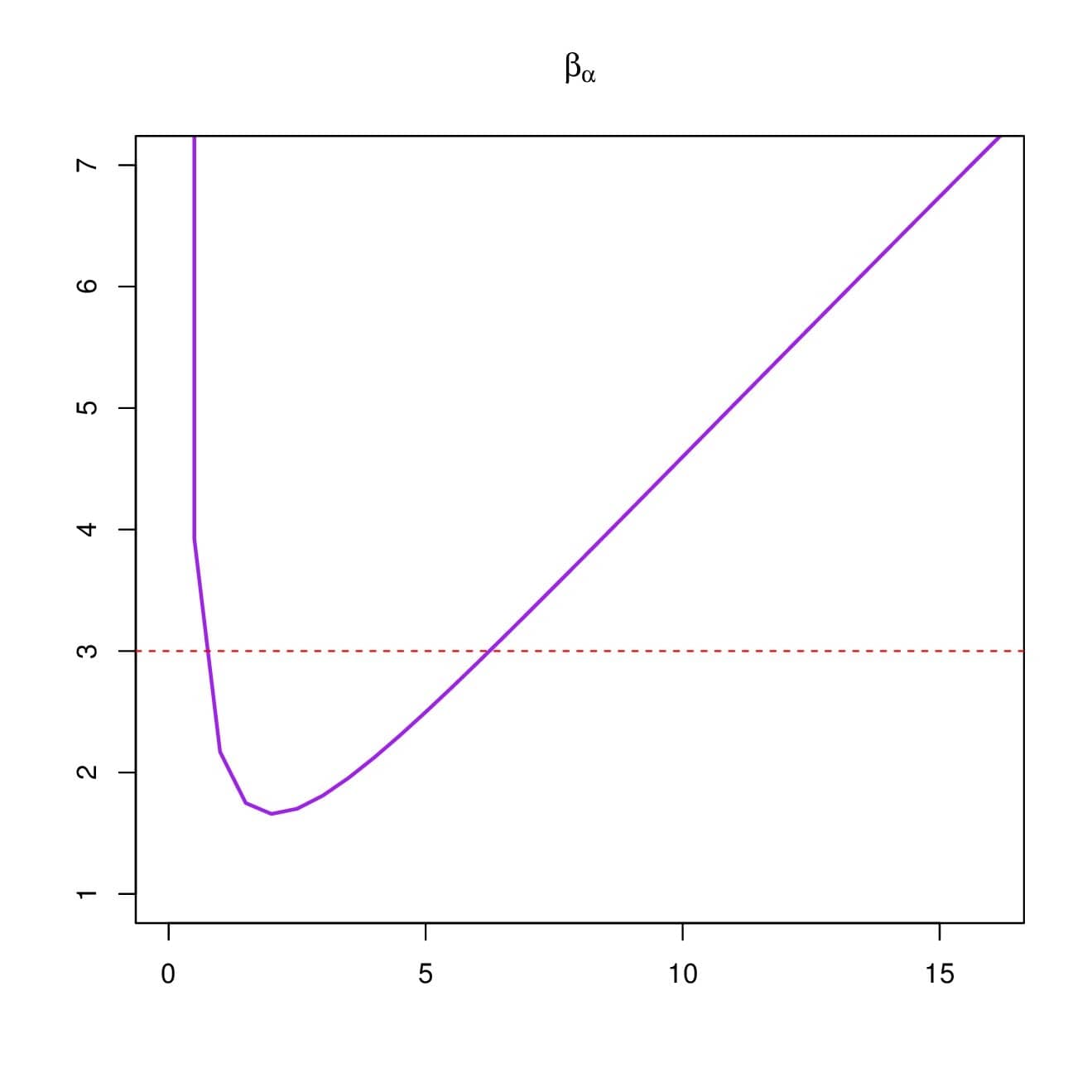
From this figure, one can remark that \(\gamma_{\alpha}\) is a strictly decreasing function with respect to \(\alpha\), and can be negative or positive, meaning that the RPL distribution can be left or right skewed, respectively. Also, we note that \(\beta_{\alpha}\) is a non-monotonic function with a “skewed V” shape. In addition, it can be inferior, equal or superior to \(3\), meaning that the RPL distribution may be platykurtic, mesokurtic, or leptokurtic, respectively.
We now discuss the moment generating function of the RPL distribution.
Proposition 8. Let \(X\) be a random variable with the RPL\((\alpha)\) distribution and \(t\in\mathbb{R}\). Then, the moment generating function of \(X\) is obtained as \begin{align*} M_{\alpha}(t) =e^t – \frac{t}{\alpha}\sum_{k=0}^{+\infty}\frac{t^k}{k!} \log\left(1+\frac{\alpha}{k+1}\right). \end{align*}
Proof. By using the Taylor series of the exponential function combined with Proposition 6, we get \begin{align*} M_{\alpha}(t)& =\mathbb{E}(e^{tX})=1+\sum_{k=1}^{+\infty}\frac{t^k}{k!}m_{\alpha}(k)=1+\sum_{k=1}^{+\infty}\frac{t^k}{k!} \left[ 1 – \frac{k}{\alpha}\log\left(1+\frac{\alpha}{k}\right)\right] \\ & =1+\sum_{k=1}^{+\infty}\frac{t^k}{k!} – \frac{1}{\alpha}\sum_{k=1}^{+\infty}\frac{t^k}{(k-1)!} \log\left(1+\frac{\alpha}{k}\right)=e^t – \frac{t}{\alpha}\sum_{k=0}^{+\infty}\frac{t^k}{k!} \log\left(1+\frac{\alpha}{k+1}\right). \end{align*} The desired formula is obtained.
As a consequence of Proposition 8, we have
\begin{align*} M_{\alpha}(r,t)=\mathbb{E}(X^r e^{tX})=\frac{\partial^r }{\partial t^r}M_{\alpha}(t)&= e^t – \frac{1}{\alpha}\sum_{k=r-1}^{+\infty}\frac{k+1}{(k-r+1)!} t^{k-r+1} \log\left(1+\frac{\alpha}{k+1}\right). \end{align*} This formula can be applied for any chosen value of \(t\). The following relationship can be used to obtain the \(r \)th ordinary moment: \(m_{\alpha}(r)=M_{\alpha}(r,0)\).The incomplete moments of the RPL distribution are now expressed.
Proposition 9. Let \(X\) be a random variable with the RPL\((\alpha)\) distribution, \(r\) be a positive integer, and \(X_t\) be the truncated version of \(X\) at a threshold \(t\) with \(t\in [0,1]\). Then, the \(r\)th incomplete moment of \(X\) at \(t\) is obtained as the \(r\)th ordinary moment of \(X_t\), that is \begin{align*} m_{\alpha}(r, t)=\mathbb{E}(X_t^r)= t^rF_{\alpha}(t)-\frac{r}{\alpha} \left\lbrace Ei[ (\alpha+r)\log(t)]- Ei[ r\log(t)] \right\rbrace, \end{align*} where \(Ei(x)\) is the exponential integral defined by \[Ei(x)=\int_{-\infty}^x\frac{e^{t }}{t}dt, \quad x\in \mathbb{R}^*.\]
Proof. We proceed as for the proof of Proposition 6. We have \[m_{\alpha}(r, t)=\int_{-\infty}^{t}x^r f_{\alpha}(x)dx=\frac{1}{\alpha}\int_{0}^{t}x^{r-1} \frac{\alpha x^{\alpha}\log(x)+1-x^{\alpha}}{(\log(x))^2} dx.\] Now, let us consider the following function: \begin{align*} \Psi_{r}(\alpha,t)&=\int_{0}^{t}x^{r-1} \frac{\alpha x^{\alpha}\log(x)+1-x^{\alpha}}{(\log(x))^2} dx, \end{align*} with \(\Psi_{r}(\alpha,t)=0\) for \(\alpha=0\). By applying the Leibnitz integral rule, we get \begin{align*} \frac{\partial}{\partial \alpha}\Psi_{r}(\alpha,t)&=\frac{\partial}{\partial \alpha} \int_{0}^{t}x^{r-1} \frac{\alpha x^{\alpha}\log(x)+1-x^{\alpha}}{(\log(x))^2} dx =\int_{0}^{t}x^{r-1} \frac{1}{(\log(x))^2}\frac{\partial}{\partial \alpha} (\alpha x^{\alpha}\log(x)+1-x^{\alpha}) dx\\ & = \int_{0}^{t}x^{r-1}\frac{1}{(\log(x))^2} \times \alpha x^{\alpha } (\log(x))^2dx= \alpha \int_{0}^{t}x^{r+\alpha-1}dx=\frac{\alpha}{r+\alpha}t^{r+\alpha}. \end{align*} Now, by an integration with respect to \(\alpha\) and suitable changes of variables, we obtain \begin{align*} \int_{0}^{\alpha}\frac{u}{r+u}t^{r+u} du&= t^{r}\int_{0}^{\alpha} t^{u}du-r \int_{0}^{\alpha} \frac{t^{r+u}}{r+u}du \\ & =t^r\frac{t^{\alpha}-1}{\log(t)}-r \int_{r}^{\alpha+r} \frac{t^{v}}{v}dv =t^r\frac{t^{\alpha}-1}{\log(t)}-r \int_{r\log(t)}^{(\alpha+r)\log(t)} \frac{e^{w}}{w}dw \\ & = \alpha t^rF_{\alpha}(t)-r \left\lbrace Ei[ (\alpha+r)\log(t)]- Ei[ r\log(t)] \right\rbrace. \end{align*} Therefore, \(\Psi_{r}(\alpha,t)= \alpha t^rF_{\alpha}(t)-r \left\lbrace Ei[ (\alpha+r)\log(t)]- Ei[ r\log(t)] \right\rbrace+c\), where \(c\) denotes a certain constant satisfying \(\Psi_{r}(0,t)=0\), that is, \(c=0\). Therefore \[\Psi_{r}(\alpha,t)= \alpha t^rF_{\alpha}(t)-r \left\lbrace Ei[ (\alpha+r)\log(t)]- Ei[ r\log(t)] \right\rbrace.\] Hence \[m_{\alpha}(r, t)=\frac{1}{\alpha}\Psi_{r}(\alpha,t)=t^rF_{\alpha}(t)-\frac{r}{\alpha} \left\lbrace Ei[ (\alpha+r)\log(t)]- Ei[ r\log(t)] \right\rbrace,\] ending the proof of Proposition 9.
From Proposition 9, we refind the \(r\)th ordinary moment of \(X\) by the limit technique; since
\begin{align*} t^rF_{\alpha}(t)\underset{t\rightarrow 1}{=}1, \quad Ei[ (\alpha+r)\log(t)]- Ei[ r\log(t)] \underset{t\rightarrow 1}{=}\log\left( 1+\frac{\alpha}{r}\right), \end{align*} we obtain \begin{align*} m_{\alpha}(r)\underset{t\rightarrow 1}{=}m_{\alpha}(r, t)=1 – \frac{r}{\alpha}\log\left(1+\frac{\alpha}{r}\right). \end{align*} We mention that the incomplete moments are used in a variety of essential probability functions, including the residual life function and its ordinary moments, the respected residual life function and its ordinary moments, the Lorenz, Zenga and Bonferroni curves, and so on. On this topic, we may refer to [32].We intend to demonstrate that the RPL distribution can provide better results than the comparable one-parameter UPL and Po distributions for some types of data and with the use of MLEs. We recall that the functions in Equations (2) and (1) specified these two last distributions, respectively. For comparison, we use established statistical criteria, such as the Akaike information criterion (AIC), corrected Akaike information criterion (AICc) and Bayesian information criterion (BIC), defined by \(\text{AIC} = -2 \log L_{\hat{\alpha}} + 2 k\), \(\text{AICc}=\text{AIC}+2 k (k+1)/(n-k-1)\) and \(\text{BIC} = -2 \log L_{\hat{\alpha}}+ k \log(n)\), respectively, where \(k\) is the number of parameters to be estimated. For the considered distributions, since there is only one parameter, we take \(k=1\). The distribution with the smallest AIC, AICc, or BIC is considered to have the best fit of the data.
Here, we generate four different data sets presenting U or J shapes. More precisely, each data set contains \(200\) values which are realisations of the following random variable: \(X=1/(1+Y)\), where \(Y\) is a random variable with the Pareto distribution specified by the following pdf: \(f^{\flat}_{\upsilon, \theta}(x)=\theta \upsilon^{\theta}x^{-(\theta+1)}\), \(x\ge \upsilon\), and \(f^{\flat}_{\upsilon, \theta}(x)=0\) for \(x0\) and \(\theta>0\). For the \(j\)th data set, called Data set \(j\), we consider the following parameters: \(\upsilon=2^{-(j+2)}\) and \(\theta=(j+2)^{-1/2}\) with \(j=1,2,3,4\).
The considered criteria for the three distributions are given in Table 2, for each data set. In all the calculations, the R software is used, and all the codes are available upon author request.
| Data set 1 | MLE \(\hat \alpha\) | AIC | AICc | BIC |
|---|---|---|---|---|
| RPL | 4.612479 | -36.65037 | -36.63017 | -33.35205 |
| UPL | 2.148819 | -26.77903 | -26.75883 | -23.48071 |
| Po | 1.374657 | -16.26337 | -16.24317 | -12.96506 |
| Data set 2 | ||||
| RPL | 6.653810 | -105.23541 | -105.21521 | -101.93710 |
| UPL | 6.294888 | -57.57819 | -57.55799 | -54.27987 |
| Po | 1.344703 | -13.93269 | -13.91249 | -10.63437 |
| Data set 3 | ||||
| RPL | 11.298643 | -225.40800 | -225.38780 | -222.10968 |
| UPL | 16.288507 | -174.03556 | -174.01536 | -170.73724 |
| Po | 1.696079 | -45.16569 | -45.14549 | -41.86737 |
| Data set 4 | ||||
| RPL | 16.280371 | -301.34203 | -301.32183 | -298.04371 |
| UPL | 34.643019 | -229.43869 | -229.41849 | -226.14037 |
| Po | 1.471506 | -24.34491 | -24.32471 | -21.04659 |
In this table, the smallest values of AIC, AICc, and BIC are obtained for the RPL distribution; it can be considered as the best.
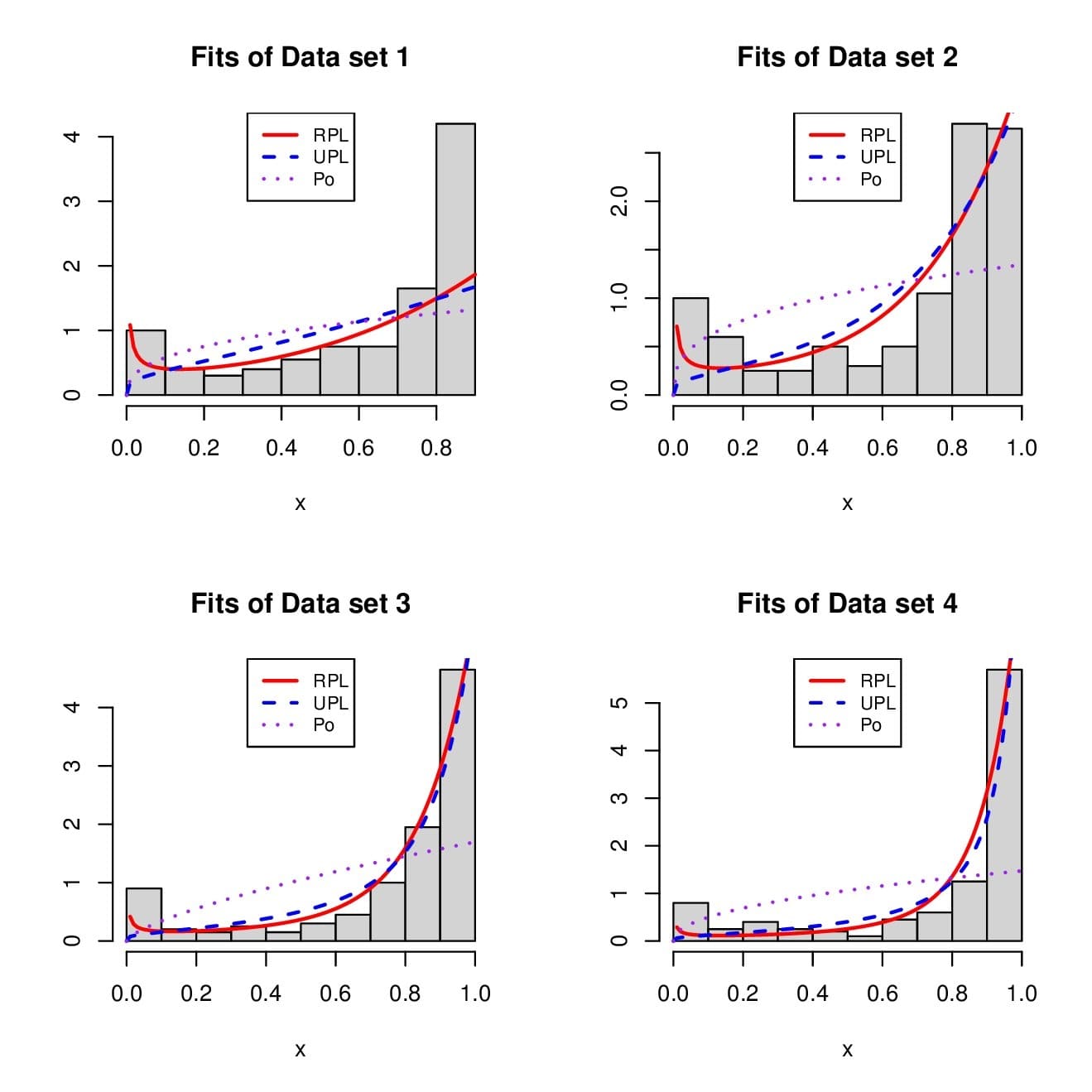
In the setting of the RPL distribution, based on the MLE \(\hat \alpha\), the estimated pdf is given by \(\hat f(x)=f_{\hat \alpha}(x)\). We can define the estimated pdfs of the UPL and Po distributions in a similar manner. Figure 8 shows how these estimated pdfs fit the histogram of the data.
From this figure, we see that the RPL distribution has well captured the U or J shapes of the histograms, and especially the data to the left corresponding to \(x\in (0, 0.1)\), which is not the case of the two competitors.
Proposition 10. Let \(\alpha>0\). Then the following equality holds: \begin{align*} \int_{0}^{1}\frac{\log(1-x)}{x (\log(x))^2} \left[x^{\alpha}(1-\alpha \log(x))-1\right]dx=& \alpha \gamma + \log[\Gamma(\alpha+1)], \end{align*} where \(\gamma\) is the Euler constant and \(\Gamma(x)\) is the standard gamma function.
Proof. We will prove this result by using the moments of the RPL distribution. For any random variable \(X\) following the RPL distribution and any positive integer \(k\), it comes from Proposition 6 that \[\frac{1}{k}\mathbb{E}(X^k)=\frac{1}{k} – \frac{1}{\alpha}\log\left(1+\frac{\alpha}{k}\right).\] It follows from this relation, the Lebesgue dominated convergence theorem and the series expansion of the logarithmic function that
A new integral expression of the Euler constant comes from Proposition 10; by taking \(\alpha=1\), we get
\begin{align*} \gamma = \int_{0}^{1}\frac{\log(1-x)}{x (\log(x))^2} \left[x(1-\log(x))-1\right]dx. \end{align*} As far as we know, this integral form of the Euler constant is not listed in the literature, at least under this form. In particular, it dont appear in the indispensable book of [34]. Some relationships with existing integrals are formulated below.The next result is derived to Proposition 10, and also appears in [35].
Proposition 11. Let \(\alpha>0\). Then the following equality holds: \begin{align*} \int_{0}^{1}\frac{1}{(1-x)\log(x)}[\alpha\log(x) + 1 -x^{\alpha}]dx= \alpha \gamma + \log[\Gamma(\alpha+1)]. \end{align*}
Proof. We follow the spirit of the proof of Proposition 10, with the same notations. By using Equations (6) and (4), applying an integration by part and using \(S_{\alpha}(x)\underset{x\rightarrow 1}{\sim}\alpha(1-x)/2\), we get \begin{align*} \gamma + \frac{1}{\alpha}\log[\Gamma(\alpha+1)]&= \sum_{k=1}^{+\infty}\left[\frac{1}{k} – \frac{1}{\alpha}\log\left(1+\frac{\alpha}{k}\right) \right]=\mathbb{E}\left(-\log(1-X)\right) = \int_{0}^{1}[-\log(1-x)]f_{\alpha}(x)dx\\ & = [-\log(1-x)](-S_{\alpha}(x)) \mid_{x=0}^1+\int_{0}^{1}\frac{1}{1-x}S_{\alpha}(x)dx\\ & =0+ \int_{0}^{1}\frac{1}{1-x}\frac{\alpha\log(x) + 1 -x^{\alpha}}{\alpha\log(x)}dx, \end{align*} implying that \begin{align*} &\int_{0}^{1}\frac{1}{(1-x)\log(x)}[\alpha\log(x) + 1 -x^{\alpha}]dx= \alpha \gamma + \log[\Gamma(\alpha+1)]. \end{align*} The desired outcome is achieved.
In [35], the proof is completely different; it is based on a parametric derivative-sum-integral technique.
The above findings may be used for a variety of purposes, beyond the scope of the article.
The author declares no conflict of interest.
The data required for this research are simulated data. The code is available on request from the author.
No funding is available for this research.
The author is thankful to the two anonymous referees for their constructive comments.