A continuous two-step block method with two hybrid points for the numerical solution of first order ordinary differential equations is proposed. The approximate solution in form of power series and its first ordered derivative are respectively interpolated at the point \(x=0\) and collocated at equally spaced points in the interval of consideration. The application of the method involves using the main scheme derived together with the additional schemes simultaneously to obtain the solution to the problem at the grid points. The analysis of the method and the results obtained from the examples considered show that the method is consistent, zero-stable, convergent and of high accuracy.
Ordinary Differential Equations (ODEs) are important models derived from real-life problems and other natural phenomena. In particular, many problems in engineering, biology, physics and other social sciences have been modelled resulting in ordinary differential equations, [1,2,3].
The main focus of this paper is to consider an accurate approximate method for the solution of general first order initial value problem of the form
where \(f(x,y)\) is continuous and satisfies the existence and uniqueness of solution theorem, [4]. Predictor-corrector methods for solving ordinary differential equations of the form (1) proposed by [5] has some demerits which necessitated the introduction of hybrid block methods. Hybrid methods were initially introduced to overcome zero-stability barrier that occurred in block methods, Dahlquist (1956). Apart from the ability to change step size, the benefit of the hybrid block methods is utilizing data off-step points which contributes to the accuracy of the methods, [6]. The standard collocation method at some selected points introduced by [7] was discrete in nature. However, [8] was able to show that the traditional multistep methods including the hybrid ones can be made continuous. This was done through the idea of multistep collocation scheme against the discrete schemes. Through this, better approximation at all interior points and absolute error estimates were obtained.
According to [9], the continuous linear multi-step method has greater advantage over the discrete method in that it gives better error estimation, provides a simplified form of coefficient for further analytical work at different points and guarantees easy appropriation of solutions at all interior points within the interval of integration. [10,11,12] proposed methods which were implemented in predictor-corrector mode and adopted Taylor series expansion to supply the starting value. Generally, the major setback of the predictor-corrector method is the high cost of implementation, as subroutines are very complicated to write because of the special techniques required to supply starting values, [13]. Therefore, the need to address this setback by proposing a method that melts the properties of both the block method and the predictor-corrector method cannot be over-emphasised. To solve Eq. (1), numerical methods are developed by types of Ordinary Differential Equations (ODEs) such as non-linear, linear, either stiff or non-stiff ODEs. It should be noted that by using inappropriate method for a model may lead to slow convergence or wrong solution, [14,15] observed that Methods such as Adomian decomposition method, variational iteration method, Chebyshev’s wavelet method, classical fourth-order Runge-Kutta method, homotopy perturbation method have some setbacks ranging from small convergence/implementation regions to inefficiency in terms of accuracy.
We therefore, present a self-starting continuous two-step hybrid block method with faster rate of convergence and better accuracy for the numerical integration of initial value problems of first order ordinary differential equations. In doing this, the collocation points were evenly selected in the interval of consideration.
Interpolating (4) at \(x=x_{n}\) such that \(i=0\) and collocating (5) at \(x=x_{n+i}\) for \(i={0,~\frac{1}{2},~1,~\frac{3}{2},~2}\), we have the following six equations
Solving (12) by Gaussian elimination method, we obtain the continuous variables \(a_{i}\)’s and the parameters \(\alpha_{j}\) and \(\beta_{j}\) as the following functions of \(t\).
\begin{align*}\alpha_{0}(t)&=1,\\
\beta_{0}(t)&=t-\frac{25}{12}t^{2}+\frac{35}{18}t^{3}-\frac{5}{6}t^{4}+\frac{2}{15}t^{5},\\
\beta_{\frac{1}{2}}(t)&=4t^{2}-\frac{52}{9}t^{3}+3t^{4}-\frac{8}{15}t^{5},\\
\beta_{1}(t)&=-3t^{2}+\frac{57}{9}t^{3}-4t^{4}+\frac{4}{5}t^{5},\\
\beta_{\frac{3}{2}}(t)&=\frac{4}{3}t^{2}-\frac{28}{9}t^{3}+\frac{1}{2} t^{4}-\frac{8}{15}t^{5},\end{align*}
and
\[\beta_{2}(t)=-\frac{1}{4}t^{2}+\frac{11}{18}t^{3}-\frac{7}{4} t^{4}+\frac{2}{15}t^{5}.\]
Eq. (2) is re-written as
We evaluate \(\beta_{j}(t)\) at \(t=0,~\frac{1}{2},~1,~\frac{3}{2},~2\) and substitute the values obtained into (13) to obtain the hybrid block methods as
where \(y(x)\) is an arbitrary test function that is continuously differentiable in the interval \([a,b]\). Expanding \(y(x_{n}+jh)\), \(y'(x_{n}+jh)\) and \(y'(x_{n}+vih)\) in Taylor series about \(x_{n}\) and collecting the coefficients of \(h^{(q)}~: q=0,1,2,3,…\) to get
where \(c_{q}\) are vectors. From Eq. (19), if we can obtain that
\[c_{0}=c_{1}=c_{2}=…=c_{q}=0 : c_{q+1}\neq 0\]
then the hybrid block method (2) is said to be of order \(q\) and its error constant is \(c_{q+1}\), [16,17].
Now, expanding Eq. (14) in Taylor’s series around \(y(x=x_{n+\frac{1}{2}})\) and collecting like terms in \(h^{q}y^{(q)}(x_{n})~:q=0,1,2,3,..\) we obtain
In Eq. (21), \[c_{0}=c_{1}=c_{2}=c_{3}=c_{4}=c_{5}=0~:~ c_{6}=\frac{3h^{6}}{10240}.\]
In a similar manner, we obtained from Eqs. (15), (16) and (17) by evaluating respectively at \(y(x=x_{n+1})\), \(y(x=x_{n+\frac{3}{2}})\) and \(y(x=x_{n+2})\)
\[c_{0}=c_{1}=c_{2}=c_{3}=c_{4}=c_{5}=0~:~ c_{6}=\frac{h^{6}}{5760},\]
\[c_{0}=c_{1}=c_{2}=c_{3}=c_{4}=c_{5}=0~:~ c_{6}=\frac{3h^{6}}{10240},\]
\[c_{0}=c_{1}=c_{2}=c_{3}=c_{4}=c_{5}=c_{6}=0~:~ c_{7}=-\frac{h^{7}}{15120}.\]
Therefore, the orders of our scheme are obtained as \((5,~5,~5,~6)^{T}\) and error constants as \[\left(\frac{3}{10240},~\frac{1}{5760},~\frac{3}{10240},~-\frac{1}{15120}\right)^{T}\]
3.2. Consistency
A linear multistep method is said to be consistent if it has an order of convergence, \(q\geq 1\) [18]. The derived hybrid block method is consistent since the orders are all greater than
3.3. Zero stability
A linear multistep method of the form (2) is said to be zero stable if no roots of the first characteristic polynomial \(\rho(R)\) has modulus greater than one, and if every root of modulus one is simple, [18,19],
Eqs (14) to (17) are put in block form as
where \(A^{0}=\left[\begin{matrix}
1 & 0 & 0 & 0 \\
0 & 1 & 0 & 0 \\
0 & 0 & 1 & 0 \\
0 & 0 & 0 & 1
\end{matrix}\right]\) and \(A^{1}=\left[\begin{matrix}
0 & 0 & 0 & 1 \\
0 & 0 & 0 & 1 \\
0 & 0 & 0 & 1 \\
0 & 0 & 0 & 1
\end{matrix}\right]\).
Therefore, \[\rho(R)=det\left( R\left[\begin{matrix}
1 & 0 & 0 & 0 \\
0 & 1 & 0 & 0 \\
0 & 0 & 1 & 0 \\
0 & 0 & 0 & 1
\end{matrix}\right]-\left[\begin{matrix}
0 & 0 & 0 & 1 \\
0 & 0 & 0 & 1 \\
0 & 0 & 0 & 1 \\
0 & 0 & 0 & 1
\end{matrix}\right]\right) =det\left[\begin{matrix}
R & 0 & 0 & -1 \\
0 & R & 0 & -1 \\
0 & 0 & R & -1 \\
0 & 0 & 0 & R-1
\end{matrix}\right]\]
Implies, \(\rho(R)=R^{4}-R^{3}.\) Since \(\rho(R)=0\), so \(R^{4}-R^{3}=0.\)
Therefore, the roots of the first characteristics polynomial are \(R_{1}=R_{2}=R_{3}=0\) and \(R_{4}=1\) and
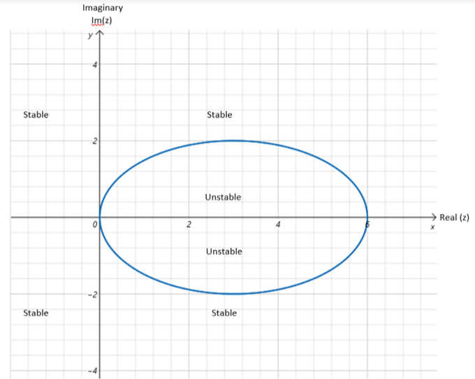
\(\rho(R)\) satisfies the condition \(|R|\leq 1\) and \(|R|=1\) is simple, then our block hybrid scheme given by Eqs. (14) – (17) is zero stable.
Figure 1. Stability region of the two-step with three hybrid points method.
3.4. Convergence
The convergence of the hybrid two-step method is considered in the light of its basic properties, that is the consistency and zero-stability; in conjunction with the fundamental theorem of Dahlquist for linear multi-step method which states that “the necessary and sufficient condition for a multi-step method to be convergent is for it to be consistent and zero-stable”, [4]. Then the hybrid block method discussed is convergent since it is consistent and zero-stable.
3.5. Numerical Implementation of the Scheme
In this section, we test the effectiveness and validity of our derived scheme by applying it to some first order differential equations. Unlike the predictor-corrector method which requires that the starting values \(y_{n+j},~j=0,~1,~2,…\) be generated first, the proposed method is self starting thereby reducing the amount of work in the computation. For error calculation, the error formula is given by
Table 1 shows the comparison between our method and the Euler method with.
Table 1. Numerical results for Example 1: Comparison between the absolute errors in our method and Euler method.
x
Exact solution
Euler method error
Our method error
0.0
1.00000
1.000000.000000
1.000000.000000
0.1
0.99010
1.000009.900e-3
0.990100.000000
0.2
0.96154
0.980001.846e-2
0.961531.000e-5
0.3
0.91743
0.941582.415e-2
0.917441.000e-5
0.4
0.86207
0.888392.632e-2
0.862070.000000
0.5
0.80000
0.825252.525e-2
0.800000.000000
0.6
0.73529
0.757152.186e-2
0.735290.000000
0.7
0.67114
0.688351.721e-2
0.671131.000e-5
0.8
0.60976
0.622021.226e-2
0.609760.000000
0.9
0.55249
0.560117.620e-3
0.552501.000e-5
1.0
0.50000
0.503643.640e-3
0.500000.000000
Example 2.[(19])
Consider the following linear Ordinary Differential Equation
\begin{equation}\label{e26}
y’=x+y, y(0)=1~:~0\leq x \leq 1.
\end{equation}
(26)
The exact solution is \(y(x)=2e^{x}-x-1\).
Table 2 shows the comparison between our method; third order Adams-Moulton (A-M) method and fourth order Milne-Simpson (M-S) method. Applying the Adams-Moulton and Milne-Simpson methods, the starting value \(y_{1}\) was determined using Taylor series method of appropriate order.
Table 2. Numerical results for Example 2: Comparison between the absolute errors in our method and other methods in literature .
x
Exact solution
Error in our method
Error in A-M
Error in M-S
0.0
1.0000000
0.0000000
0.0000000
0.0000000
0.1
1.1103418
0.0000000
8.5.000e-6
2.0000e-7
0.2
1.2428055
0.0000000
3.0000e-7
2.0000e-7
0.3
1.3997176
1.0000e-7
1.1200e-5
1.0000e-7
0.4
1.5836494
0.0000000
2.4300e-5
5.0000e-7
0.5
1.7974425
0.0000000
4.0200e-5
5.0000e-7
Example 3. Consider the nonlinear Ordinary Differential Equation
Table 4 shows the comparison between our method; Block Method with One Hybrid Point (BM1HP) by [22], One-Sixth Hybrid Block Method (OSHBM) derived by using the Chebyshev polynomials by [21] and One-Step Block Method with Three Hybrid (OSBM3H) points by [6].
Table 4. Numerical results for Example 4: Comparison between the absolute errors in our method and other methods in literature.
x
Error in our method
Error in OSBM3H
Error in BM1HP
Error in OSHBM
0.0
0.0000000
0.0000000
0.0000000
0.0000000
0.01
1.61332E-14
1.61332E-10
2.82900E-7
1.55825E-6
0.02
2.14045E-14
2.14045E-10
4.04578E-7
2.39975E-6
0.03
2.22905E-14
2.22905E-10
4.47254E-7
2.83045E-6
0.04
2.14208E-14
2.14208E-10
4.50903E-7
3.02094E-6
0.05
1.99082E-14
1.99082E-10
4.35625E-7
3.06956E-6
0.06
1.82326E-14
1.82326E-10
4.11764E-7
3.03457E-6
0.07
1.65980E-14
1.65980E-10
3.84699E-7
2.95115E-6
0.08
1.50853E-14
1.50853E-10
3.57218E-7
2.84088E-6
0.09
1.37194E-13
1.37194E-10
3.30725E-7
2.71713E-6
0.10
1.25003E-13
1.25003E-10
3.05879E-7
2.58816E-6
4. Conclusion
A two-step block method with two hybrid points for the numerical solution of first order ordinary differential equations has been proposed and discussed. The method was derived through interpolation of the assumed power series solution at the point \(x=x_{n}\) and collocation of its first ordered derivative at equally spaced points in the interval of consideration. The consistency, zero-stability and applicability of the proposed method were considered and well discussed. The analysis of the method showed that it is convergent since consistency and zero-stability properties are satisfied. Numerical results as presented in Tables 1-4 show that the method performs better than most of the existing methods in literature. Furthermore, the method produces results that are very close to the exact solutions for all the problems considered.
Author Contributions
All authors contributed equally in this paper. All authors read and approved the final version of this paper.
Conflicts of Interest
The authors declare no conflict of interest.
Data Availability
All data required for this research is included within this paper.
Funding Information
We do not have funding for this paper.
References
Odejide, S. A., & Adeniran, A. O. (2012). A hybrid linear collocation multistep scheme for solving first order initial value problems. Journal of the Nigerian Mathematical Society, 31(1-3), 229-241. [Google Scholor]
Nathaniel, K., Geoffrey, K., & Joshua, S. (2021). Continuous one step linear multi-step hybrid block method for the solution of first order linear and nonlinear initial value problem of ordinary differential equations. In Recent Developments in the Solution of Nonlinear Differential Equations. IntechOpen. [Google Scholor]
Soomro, H., Daud, H., & Zainuddin, N. (2021, July). Convergence of the 3-point block backward differentiation formulas with off-step point for stiff ODEs. In Journal of Physics: Conference Series (Vol. 1943, No. 1, p. 012137). IOP Publishing. [Google Scholor]
Henrici, P. (1962). Discrete Variable Methods in Ordinary Differential Equations. Wiley, New York. [Google Scholor]
Milne, W. E. (1953). Numerical Solutions of Differential Equations. John Wiley & Sons, New York. [Google Scholor]
Kashkari, B. S., & Syam, M. I. (2019). Optimization of one step block method with three hybrid points for solving first-order ordinary differential equations. Results in Physics, 12, 592-596. [Google Scholor]
Lanczos, C. (1965). Applied Analysis. Prentice Hall, New Jersey. [Google Scholor]
Ortiz, E. L. (1969). The Tau method. SIAM Journal of Numerical Analysis, 6, 480 – 492. [Google Scholor]
Awoyemi, D. O. (1999). A class of continuous methods for general second order initial value problems in ordinary differential equations. International Journal of Computer Mathematics, 72(1), 29-37. [Google Scholor]
Anake, T. A., Awoyemi, D. O., & Adesanya, A. O. (2012). One-step implicit hybrid block method for the direct solution of general second order ordinary differential equations. IAENG International Journal of Applied Mathematics, 42(4), 224 – 228. [Google Scholor]
Adesanya, A. O., Anake, T. A., & Oghonyon, J. G. (2009). Continuous implicit method for the solution of general second order ordinary differential equations. Journal of the Nigerian Association of Mathematical Physics, 15, 71-78. [Google Scholor]
Kayode, S. J., & Awoyemi, D. O.(2010). A multi derivative collocation implicit method for fifth order ordinary differential equation. Journal of Mathematics and Statistics, 6(1), 60-63. [Google Scholor]
James, A. A., Adesanya, A. O., Odekunle, M. B., & Yakubu, D. G. (2014). New hybrid block predictor, hybrid corrector integrator for the solution of first order IVPs of ODEs. In Proceedings of the Mathematical Association of Nigerian Annual National Conference.[Google Scholor]
Soomro, H., Zainuddin, N., & Daud, H. (2021, July). Convergence properties of 3-point block Adams method with one off-step point for ODEs. In Journal of Physics: Conference Series(Vol. 1988, No. 1, p. 012038). IOP Publishing. [Google Scholor]
Tumba, P., Sunday, J., & El-Yaqub, M. (2021, May). An efficient algorithm for the computation of Riccati differential equations. In Science Forum (Journal of Pure and Applied Sciences) (Vol. 21, No. 1, pp. 241-241). Faculty of Science, Abubakar Tafawa Balewa University Bauchi. [Google Scholor]
Ola Fatunla, S. (1991). Block methods for second order ODEs. International Journal of Computer Mathematics, 41(1-2), 55-63. [Google Scholor]
Lambert, J. D. (1973). Computational Method in ODEs. John Wiley & Sons, New York. [Google Scholor]
Singh, G., Kanwar, V., & Bhatia, S. (2013). Exponentially fitted variants of the two-step Adams-Bashforth method for the numerical integration of initial value problems. Journal of Application and Applied Mathematics, 8(2), 741-755. [Google Scholor]
Jain, M. K., Iyengar, S. R. K., & Jain, R. K. (2012). Numerical Methods for Scientific and Engineering Computation (Sixth Edition). New Age International Publishers, Delhi, India. [Google Scholor]
Yahaya, Y. A., & Tijjani, A. A. (2015). Formulation of corrector methods from 3-step hybrid Adams type methods for the solution of first order ordinary differential equations. International Journal of Applied Mathematical Research, 3(4), 102-107. [Google Scholor]
Rufai, M. A., Duromola, M. K., & Ganiyu, A. A. (2016). Derivation of one-sixth hybrid block method for solving general first order ordinary differential equations. IOSR Journal of Mathematics, 12(5), 20-27. [Google Scholor]
Fotta, A. U., Alabi, T. J., & Abdulqadir, B. (2015). Block method with one hybrid point for the solution of first order initial value problems of ordinary differential equations. International Journal of Pure and Applied Mathematics, 103(3), 511-521. [Google Scholor]